Dimensionality reduction: fs_pca() and fs

fs_pca() and fs_svd() do not select features. They replace the original columns with a few new ones, each a linear combination of all the inputs. You still have to measure every variable, and the components are chosen without reference to any outcome. The highest-variance directions need not be the ones that predict anything.

Both functions return a plain list rather than an fs_result.

`fs_pca()`

fs_pca() runs a PCA on the numeric columns of a data frame. Character and factor columns are kept aside as labels. Incomplete rows and zero-variance columns are dropped before the decomposition, and meta records what was used.

pca <- fs_pca(iris, num_pc = 2, label_col = "Species")
names(pca)
#> [1] "pc_loadings"   "pc_scores"     "var_explained" "pca_df"       
#> [5] "meta"          "plot"
pca$var_explained
#> [1] 0.7296245 0.2285076
pca$pc_loadings
#>                     PC1         PC2
#> Sepal.Length  0.5210659 -0.37741762
#> Sepal.Width  -0.2693474 -0.92329566
#> Petal.Length  0.5804131 -0.02449161
#> Petal.Width   0.5648565 -0.06694199
head(pca$pca_df)
#>          PC1        PC2 Species
#>        <num>      <num>  <fctr>
#> 1: -2.257141 -0.4784238  setosa
#> 2: -2.074013  0.6718827  setosa
#> 3: -2.356335  0.3407664  setosa
#> 4: -2.291707  0.5953999  setosa
#> 5: -2.381863 -0.6446757  setosa
#> 6: -2.068701 -1.4842053  setosa
pca$meta$n_rows_used
#> [1] 150

Reading the output

var_explained is the share of the total variance each retained component carries. With two components out of four it sums to less than 1.
pc_loadings holds the eigenvectors (prcomp()’s rotation), one row per input column. Signs are arbitrary. A component and its negation are the same component.
pc_scores and pca_df hold the coordinates of each observation.

By default columns are centered and scaled (scale_data = TRUE), so the PCA is on the correlation matrix. Leave that on unless the columns share meaningful units. Otherwise the column with the largest variance dominates.

Plotting

A ggplot of PC1 against PC2 is built whenever a label_col is supplied, two or more components are kept, and ggplot2 is installed. plot = TRUE also prints it:

pca$plot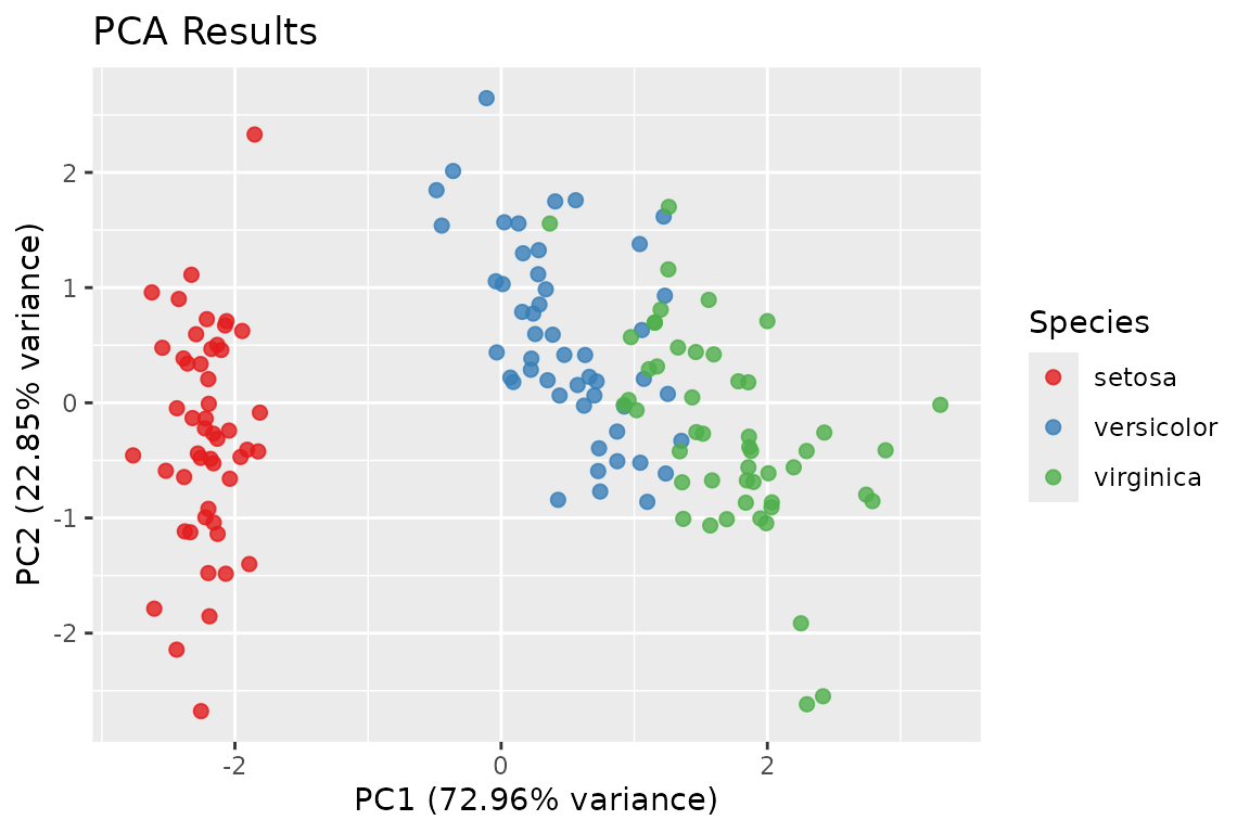

Large data

Below 10 million cells, fs_pca() uses stats::prcomp(). At or above that size it uses bigstatsr::big_SVD() on a temporary file-backed matrix, if bigstatsr is installed, and computes only the requested components. In that case the total-variance denominator is computed from column statistics, so var_explained still means share of the whole.

`fs_svd()`

fs_svd() is the lower-level tool. It takes a numeric matrix x and returns singular values and vectors:

m <- as.matrix(mtcars)
s <- fs_svd(m, n_singular_values = 3, scale_input = TRUE)
round(s$singular_values, 3)
#> [1] 14.313  9.064  4.409
dim(s$left_singular_vectors)
#> [1] 32  3
dim(s$right_singular_vectors)
#> [1] 11  3

scale_input = TRUE (the default) centers and scales the columns first, so the triplets factorize scale(x), not x. The squared singular values divided by n - 1 are the PCA eigenvalues of the scaled data:

all_sv <- fs_svd(m)$singular_values
round(all_sv^2 / (nrow(m) - 1), 4)[1:3]
#> [1] 6.6084 2.6505 0.6272
round(prcomp(m, scale. = TRUE)$sdev^2, 4)[1:3]
#> [1] 6.6084 2.6505 0.6272

Exact or approximate

svd_method = "auto" uses base::svd() unless you ask for fewer singular values than min(dim(x)) and the matrix is larger than svd_threshold (100) in its smaller dimension. In that case it uses RSpectra::svds(), which computes only the leading triplets. svd_method = "approx" forces the approximate solver when it is applicable.

set.seed(1)
big <- matrix(rnorm(400 * 150), 400, 150)
approx <- fs_svd(big, n_singular_values = 5, svd_method = "approx")
exact  <- fs_svd(big, n_singular_values = 5, svd_method = "exact")
all.equal(approx$singular_values, exact$singular_values, tolerance = 1e-6)
#> [1] TRUE

Singular vectors are unique only up to sign, so compare them with abs() or through reconstructions, not element by element.

Dimensionality reduction: fs_pca() and fs_svd()