bmbeR walks a regression model through the stages of a Bayesian workflow (Gelman et al., 2020) and treats the prior as part of the model at every stage:
- Specify priors on the scale of the data.
- Check what they imply before seeing the outcome (prior predictive check).
- Fit the model and verify the computation (R-hat, effective sample size, divergences, E-BFMI).
- Quantify how much the prior influenced the result (power-scaling sensitivity).
- Evaluate predictions with proper scoring rules.
- Report each step in a checklist aligned with the Bayesian Analysis Reporting Guidelines (Kruschke, 2021).
Models are fitted with rstanarm, so every result is an
ordinary stanreg object that works with the rest of the
Stan ecosystem.
library(bmbeR)
data(kidiq, package = "rstanarm")
head(kidiq)
#>   kid_score mom_hs    mom_iq mom_age
#> 1        65      1 121.11753      27
#> 2        98      1  89.36188      25
#> 3        85      1 115.44316      27
#> 4        83      1  99.44964      25
#> 5       115      1  92.74571      27
#> 6        98      0 107.90184      18
The kidiq data (Gelman & Hill, 2007) record the test
scores of 434 children together with their mothers’ IQ and whether the
mother finished high school. We hold out a test set to evaluate
predictions at the end.
set.seed(42)
test_rows <- sample(nrow(kidiq), 100)
train <- kidiq[-test_rows, ]
test  <- kidiq[test_rows, ]
1. Specify priors
Priors only make sense relative to the units of the data. Children’s test scores are on an IQ-like scale (mean about 100, SD about 15), so:
- the intercept is the expected score of a child
whose mother has average IQ and schooling (rstanarm puts the intercept
prior at the predictor means, so you don’t have to centre the predictors
yourself):
normal(100, 20); - a one-point increase in the mother’s IQ is unlikely to change the
child’s score by more than about two points:
normal(0, 1)formom_iq; - finishing high school might plausibly shift scores by up to about 20
points:
normal(0, 10)formom_hs; - the residual SD is probably of the order of 15 points:
exponential(1/15).
priors <- prior_config(
  intercept = prior_spec("normal", location = 100, scale = 20),
  slope     = prior_spec("normal", location = 0, scale = c(1, 10)),
  aux       = prior_spec("exponential", rate = 1 / 15)
)
priors
#> <bmb_prior_config>
#>   intercept : normal(location = 100, scale = 20)
#>   slope     : normal(location = 0, scale = [1, 10])
#>   aux       : exponential(rate = 0.0667)
If you have no substantive knowledge to encode, leave components as
NULL to use rstanarm’s autoscaled weakly informative
defaults, or derive priors from data with
empirical_bayes_priors() (see the article on
Data-informed priors).
2. Check the priors before fitting
A prior predictive check simulates data from the priors alone. Test scores cannot be negative, and scores above 200 would be absurd, so we declare that range as plausible:
pc <- prior_predictive_check(train, kid_score ~ mom_iq + mom_hs,
                             prior_config = priors,
                             plausible_range = c(0, 200), refresh = 0)
pc
#> <bmb_prior_check> 200 simulated data sets of 334 observations (gaussian family)
#>   Observed outcome range     : [20, 136]
#>   Prior predictive quantiles : 1%: 16.89 | 5%: 48.73 | 50%: 99.92 | 95%: 152.9 | 99%: 180
#>   Mean of simulated data (5%, 50%, 95%): 67.75, 100.1, 132.1
#>   Share of simulated values outside plausible range [0, 200]: 0.9%
plot(pc)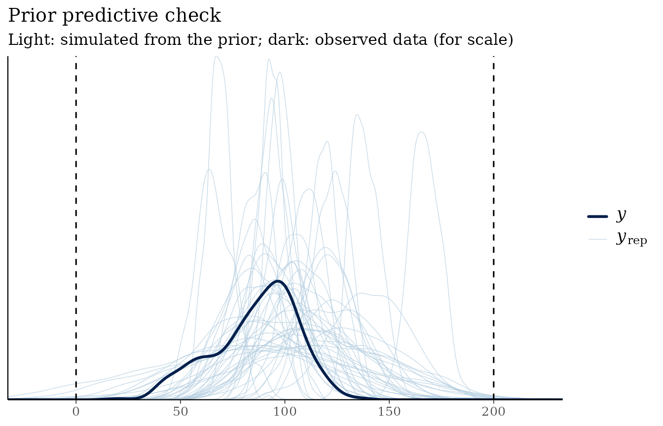
The simulated data sets are wider than the observed data, as weakly informative priors should make them, but only 0.9% of simulated values fall outside the plausible range.
3. Fit the model and verify the computation
fit <- fit_model_with_prior(train, kid_score ~ mom_iq + mom_hs,
                            prior_config = priors,
                            chains = 4, iter = 1000, refresh = 0)
attr(fit, "bmb_convergence")
#> <bmb_convergence> PASSED  (4 chains, 2000 post-warm-up draws)
#>   Criteria: R-hat <= 1.01; bulk/tail-ESS >= 400; divergences <= 0; E-BFMI >= 0.3
#>   Max R-hat: 1.003 | min bulk-ESS: 2237 | min tail-ESS: 1271
#>   Divergences: 0 | max-treedepth hits: 0 | min E-BFMI: 0.98
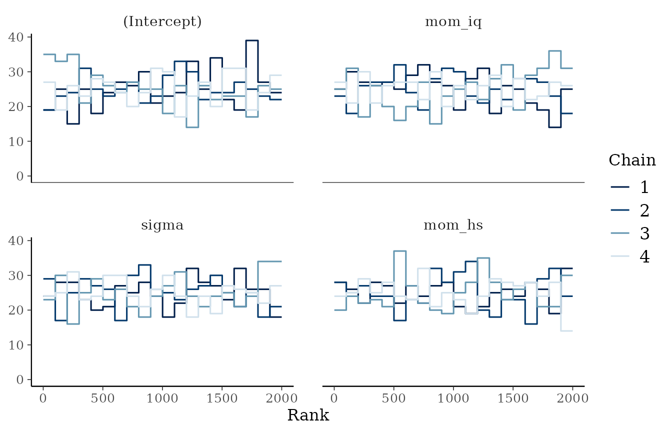
fit_model_with_prior() runs
check_convergence() automatically with the criteria of
Vehtari et al. (2021): rank-normalised R-hat of at most 1.01, bulk- and
tail-ESS of at least 100 per chain, no divergent transitions and E-BFMI
of at least 0.3. If a check fails it warns and still returns the fit so
you can investigate. Rank plots show mixing problems more clearly than
trace plots:
4. How much did the prior matter?
plot_prior_posterior() overlays each prior on its
posterior:
plot_prior_posterior(fit)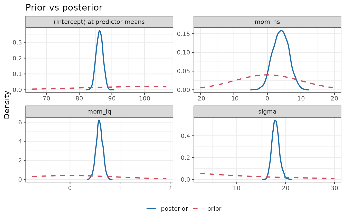
prior_sensitivity() quantifies the same question without
refitting, by power-scaling the prior and the likelihood (Kallioinen et
al., 2023):
sens <- prior_sensitivity(fit)
sens
#> <bmb_prior_sensitivity> power-scaling diagnostics (2000 draws, threshold 0.05)
#>     variable   mean    sd contraction prior_mean_sens prior_sd_sens
#>  (Intercept) 86.223 1.028       0.997           0.040        -0.007
#>       mom_iq  0.588 0.066       0.996          -0.016        -0.005
#>       mom_hs  3.975 2.344       0.945          -0.087        -0.025
#>        sigma 17.954 0.731       0.998          -0.057        -0.008
#>  lik_mean_sens lik_sd_sens conflict_z         diagnosis
#>          0.009      -0.534      0.333                 -
#>          0.008      -0.458     -0.176                 -
#>          0.101      -0.393     -0.439 informative prior
#>         -0.279      -0.588     -0.407 informative prior
#>
#> Flagged parameters:
#>   mom_hs               informative prior
#>   sigma                informative prior
#>
#> Finite perturbations: posterior mean shift, in posterior SDs, when the prior or
#> likelihood is raised to the power alpha (* = unreliable importance sampling;
#> refit with sensitivity_analysis() instead):
#>             prior a=0.8 prior a=1.25 lik a=0.8 lik a=1.25
#> (Intercept) -0.01       +0.01        -0.00     +0.00
#> mom_iq      +0.00       -0.00        +0.01     +0.00
#> mom_hs      +0.02       -0.02        -0.03     +0.02
#> sigma       +0.01       -0.01        +0.08     -0.05
#> Intercept diagnostics refer to the intercept at the predictor means.
How to read the table:
-
contractionnear 1 means the data have sharpened the prior a lot. - The
*_senscolumns measure how much the posterior mean and SD respond to strengthening the prior or the likelihood (0 = not at all). -
conflict_zmeasures disagreement between prior and data in standard-error units. A parameter whose prior is influential and whose|conflict_z|is 2 or more is diagnosed as a prior-data conflict.
The diagnosis flags mom_hs (informative prior) and
sigma (informative prior): for each,
|prior_mean_sens| or |prior_sd_sens| is at
least 0.05. Every |conflict_z| is below 2, so prior and data agree. The
Prior sensitivity article shows what weakly informative,
conflicting and weakly identified cases look like.
5. Evaluate predictions
perf <- evaluate_model_performance(fit, test)
perf
#> <bmb_performance> regression, 100 test observations
#>   ELPD (log score, higher = better)        -436
#>     SE of ELPD                             6.01
#>     ELPD per observation                   -4.36
#>   RMSE of posterior mean                   18.9
#>   MAE of posterior mean                    15.8
#>   CRPS (lower = better)                    10.9
#>   Coverage of 90% predictive intervals     0.88
#>   Mean interval width                      59.1
Besides RMSE and MAE of the posterior mean, bmbeR reports two proper scoring rules, which also reward calibrated uncertainty: the held-out log predictive density (ELPD) and the continuous ranked probability score (CRPS). Coverage of the 90% predictive intervals close to 90% indicates well-calibrated uncertainty.
6. Report
report <- workflow_report(fit, prior_check = pc, sensitivity = sens,
                          performance = perf)
report
Bayesian analysis report (BARG checklist; Kruschke, 2021)
| # | Item | Status | Detail |
|---|---|---|---|
| 1 | Model | ok | kid_score ~ mom_iq + mom_hs; gaussian family, identity link; 334 observations; 3 coefficients |
| 2 | Priors | ok | user-specified: (Intercept) ~ normal(100, 20); mom_iq ~ normal(0, 1); mom_hs ~ normal(0, 10); sigma ~ exponential(rate = 0.0667) |
| 3 | Prior predictive check | ok | 90% of prior predictive values in [48.7, 153]; observed range [20, 136] |
| 4 | MCMC computation | ok | 4 chains x 1000 iterations (500 warm-up), seed 1234. Max R-hat 1.003, min bulk-ESS 2237, min tail-ESS 1271, 0 divergences. |
| 5 | Posterior summary | ok | Means, medians, SDs and 95% central credible intervals for 4 parameters (see $posterior). |
| 6 | Posterior predictive check | ok | Posterior predictive p-values: mean 0.52, sd 0.51, min 0.89, max 0.90 |
| 7 | Cross-validation (PSIS-LOO) | ok | elpd_loo = -1440.4 (SE 13.3), p_loo = 4.1; 0 observation(s) with Pareto k > 0.70 |
| 8 | Prior sensitivity | ok | Power-scaling: mom_hs (informative prior); sigma (informative prior) |
| 9 | Held-out predictive performance | ok | ELPD = -436, RMSE = 18.9, CRPS = 10.9, Coverage = 0.88 |
| 10 | Software | ok | R 4.6.2; rstanarm 2.32.2; rstan 2.32.7; bmbeR 2.1.0 |
Posterior summary
| variable | mean | median | sd | q2.5 | q97.5 | p_positive |
|---|---|---|---|---|---|---|
| (Intercept) | 24.4 | 24.4 | 6.5 | 11.8 | 36.9 | 1 |
| mom_iq | 0.588 | 0.586 | 0.0659 | 0.456 | 0.716 | 1 |
| mom_hs | 3.97 | 4 | 2.34 | -0.524 | 8.5 | 0.96 |
| sigma | 18 | 17.9 | 0.731 | 16.6 | 19.5 | 1 |
0 item(s) need attention, 0 not yet done.
Items with status check need attention and
missing items have not been done yet; printed in the
console, these show as [check] and [ -- ]. The
report computes posterior predictive p-values and PSIS-LOO
cross-validation from the fit itself, and runs
prior_sensitivity() when no sensitivity result is
supplied.
Where next
- Choosing priors: why scale matters, autoscaling, and prior predictive checks for logistic regression.
- Data-informed priors: unit-information, empirical Bayes and power priors, and why naively re-using the data is a mistake.
- Convergence diagnostics: what each criterion means and what failure looks like.
- Prior sensitivity: the theory behind the diagnostics, and refitting under alternative priors.
- Predictive evaluation: proper scoring rules and model comparison on held-out data.
References
Gelman, A., & Hill, J. (2007). Data Analysis Using Regression and Multilevel/Hierarchical Models. Cambridge University Press. https://doi.org/10.1017/CBO9780511790942
Gelman, A., Vehtari, A., Simpson, D., et al. (2020). Bayesian workflow. arXiv:2011.01808. https://doi.org/10.48550/arXiv.2011.01808
Kallioinen, N., Paananen, T., Bürkner, P.-C., & Vehtari, A. (2023). Detecting and diagnosing prior and likelihood sensitivity with power-scaling. Statistics and Computing, 34, 57. https://doi.org/10.1007/s11222-023-10366-5
Kruschke, J. K. (2021). Bayesian analysis reporting guidelines. Nature Human Behaviour, 5, 1282–1291. https://doi.org/10.1038/s41562-021-01177-7
Vehtari, A., Gelman, A., Simpson, D., Carpenter, B., & Bürkner, P.-C. (2021). Rank-normalization, folding, and localization: An improved R-hat for assessing convergence of MCMC. Bayesian Analysis, 16(2), 667–718. https://doi.org/10.1214/20-BA1221