Predictive evaluation with proper scoring rules
Source:vignettes/articles/predictive-evaluation.Rmd
predictive-evaluation.RmdA Bayesian model predicts a distribution. Scoring only the
posterior mean (RMSE, accuracy) ignores whether the model’s uncertainty
is right. Proper scoring rules reward a forecast for being both accurate
and calibrated: in expectation, they are optimised only by reporting
your true predictive distribution (Gneiting & Raftery, 2007).
evaluate_model_performance() reports:
| Metric | Outcome | Better | Notes |
|---|---|---|---|
ELPD |
all | higher | log predictive density on the test set; the out-of-sample analogue
of elpd_loo
|
CRPS |
continuous / count | lower | in the units of the outcome; reduces to absolute error for a point forecast |
Brier |
binary | lower | mean squared error of predicted probabilities |
Coverage |
continuous / count | ≈ prob
|
calibration of the predictive intervals |
AUC |
binary | higher | discrimination only (not a proper score) |
RMSE, MAE, Accuracy,
Precision, Recall, F1_Score
|
familiar point-prediction metrics |
Binary outcomes: the wells data
data(wells, package = "rstanarm")
wells$dist100 <- wells$dist / 100
set.seed(123)
test_rows <- sample(nrow(wells), 1000)
train <- wells[-test_rows, ]
test  <- wells[test_rows, ]

fit_dist <- fit_model_with_prior(train, switch ~ dist100, family = binomial(),
                                 refresh = 0)
fit_full <- fit_model_with_prior(train, switch ~ dist100 + arsenic + educ,
                                 family = binomial(), refresh = 0)
perf_dist <- evaluate_model_performance(fit_dist, test)
perf_full <- evaluate_model_performance(fit_full, test)
perf_full
#> <bmb_performance> classification, 1000 test observations
#>   ELPD (log score, higher = better)        -652
#>     SE of ELPD                             9.14
#>     ELPD per observation                   -0.652
#>   Accuracy (threshold 0.5)                 0.611
#>   Precision                                0.629
#>   Recall                                   0.784
#>   F1 score                                 0.698
#>   Brier score (lower = better)             0.23
#>   AUC                                      0.635
Classification metrics are computed from the posterior mean
probability of switching, thresholded at 0.5 (see
threshold). Accuracy ignores how confident each prediction
was; the Brier score and ELPD also penalise overconfident
probabilities.
Comparing models on the same test set
Because both models are scored on the same households, the difference in ELPD should be assessed with the standard error of the paired (per-observation) differences, not by comparing the two ELPDs and their separate standard errors:
cmp <- compare_performance(distance_only = perf_dist, full = perf_full)
cmp
#>           model      elpd elpd_diff  se_diff
#> 1          full -652.0737   0.00000 0.000000
#> 2 distance_only -678.7845 -26.71073 6.950787
The full model’s ELPD is higher by 26.7 (SE 7.0), about 4 standard errors, so adding arsenic and education improves the predictions.
Calibration
For a calibrated model, among households given a predicted probability of about 0.7, about 70% should switch. A reliability plot checks this:
p <- colMeans(rstanarm::posterior_epred(fit_full, newdata = test))
bins <- cut(p, breaks = quantile(p, 0:10 / 10), include.lowest = TRUE)
calib <- data.frame(predicted = tapply(p, bins, mean),
                    observed  = tapply(test$switch, bins, mean))
ggplot(calib, aes(predicted, observed)) +
  geom_abline(linetype = "dashed", colour = "grey50") +
  geom_point(size = 2.5, colour = "#1b6ca8") +
  coord_equal(xlim = c(0, 1), ylim = c(0, 1)) +
  labs(x = "Mean predicted probability (decile bins)", y = "Observed share switching",
       title = "Reliability plot") +
  theme_bw()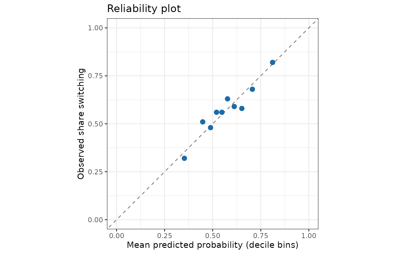
Continuous outcomes
For continuous outcomes the CRPS and interval coverage complement RMSE:
data(kidiq, package = "rstanarm")
set.seed(1)
test_rows <- sample(nrow(kidiq), 100)
fit_kid <- fit_model_with_prior(kidiq[-test_rows, ], kid_score ~ mom_iq * mom_hs,
                                refresh = 0)
evaluate_model_performance(fit_kid, kidiq[test_rows, ], prob = 0.9)
#> <bmb_performance> regression, 100 test observations
#>   ELPD (log score, higher = better)        -436
#>     SE of ELPD                             6.98
#>     ELPD per observation                   -4.36
#>   RMSE of posterior mean                   18.9
#>   MAE of posterior mean                    15.4
#>   CRPS (lower = better)                    10.8
#>   Coverage of 90% predictive intervals     0.9
#>   Mean interval width                      58.8
Coverage close to the nominal 90% means the predictive intervals are about the right width; much lower coverage signals overconfidence.
Offsets
Count models with an exposure, such as
y ~ x + offset(log(time)), need the offset of each test
observation. Offsets written in the formula are computed from the test
data. If the model was fitted with the offset argument of
stan_glm() instead, pass the test offsets with
evaluate_model_performance(fit, test, offset = log(test$time)).
Held-out data or LOO?
When no test set is available, PSIS-LOO cross-validation (Vehtari et al., 2017) estimates the same ELPD from the training data alone:
loo::loo(fit_full)
#>
#> Computed from 4000 by 2020 log-likelihood matrix.
#>
#>          Estimate   SE
#> elpd_loo  -1307.6 13.5
#> p_loo         4.2  0.2
#> looic      2615.2 27.0
#> ------
#> MCSE of elpd_loo is 0.0.
#> MCSE and ESS estimates assume independent draws (r_eff=1).
#>
#> All Pareto k estimates are good (k < 0.7).
#> See help('pareto-k-diagnostic') for details.
workflow_report() reports LOO automatically and includes
held-out metrics when you pass them via performance =.
References
Brier, G. W. (1950). Verification of forecasts expressed in terms of probability. Monthly Weather Review, 78(1), 1–3. https://doi.org/10.1175/1520-0493(1950)078%3C0001:VOFEIT%3E2.0.CO;2
Gneiting, T., & Raftery, A. E. (2007). Strictly proper scoring rules, prediction, and estimation. JASA, 102(477), 359–378. https://doi.org/10.1198/016214506000001437
Vehtari, A., Gelman, A., & Gabry, J. (2017). Practical Bayesian model evaluation using leave-one-out cross-validation and WAIC. Statistics and Computing, 27(5), 1413–1432. https://doi.org/10.1007/s11222-016-9696-4