Choosing priors: scale, autoscaling and prior predictive checks
Source:vignettes/articles/priors.Rmd
priors.RmdA prior is a statement about plausible parameter values, and a regression coefficient’s plausible values depend entirely on the units of the outcome and the predictors. This article shows what goes wrong when that is ignored, the options for getting it right, and how prior predictive checks catch problems before any model is fitted.
Why scale matters
mtcars records fuel efficiency (mpg) and
weight (wt, in 1000 lbs). We fit the same model twice: once
with mpg, and once with the outcome expressed in hundredths
of a mile per gallon (mpg * 100). Nothing about the data
has changed except the units, so the second slope should be exactly 100
times the first.
First with a fixed-scale prior,
student_t(3, 0, 2.5) on every coefficient, which was the
default in bmbeR 1.x:
d <- mtcars
d$mpg100 <- d$mpg * 100
fixed <- prior_config(intercept = prior_spec("student_t", 0, 2.5, df = 3),
                      slope     = prior_spec("student_t", 0, 2.5, df = 3))

fit_mpg    <- fit_model_with_prior(d, mpg ~ wt, prior_config = fixed,
                                   refresh = 0, on_nonconvergence = "ignore")
fit_mpg100 <- fit_model_with_prior(d, mpg100 ~ wt, prior_config = fixed,
                                   refresh = 0, on_nonconvergence = "ignore")
rbind(
  "OLS, mpg"            = coef(lm(mpg ~ wt, d)),
  "fixed prior, mpg"    = coef(fit_mpg),
  "OLS, mpg*100"        = coef(lm(mpg100 ~ wt, d)),
  "fixed prior, mpg*100" = coef(fit_mpg100)
)
#>                        (Intercept)           wt
#> OLS, mpg               37.28512617   -5.3444716
#> fixed prior, mpg       36.74066218   -5.1962046
#> OLS, mpg*100         3728.51261673 -534.4471573
#> fixed prior, mpg*100   -0.07467113    0.1569807
On the original scale the prior is harmless. On the rescaled outcome
the same prior says “the slope is almost certainly within a few units of
zero”, while the data say it is around −530. The prior wins, and the
model attributes the relationship to noise; the sigma panel
below shows the inflated residual SD.
plot_prior_posterior(fit_mpg100)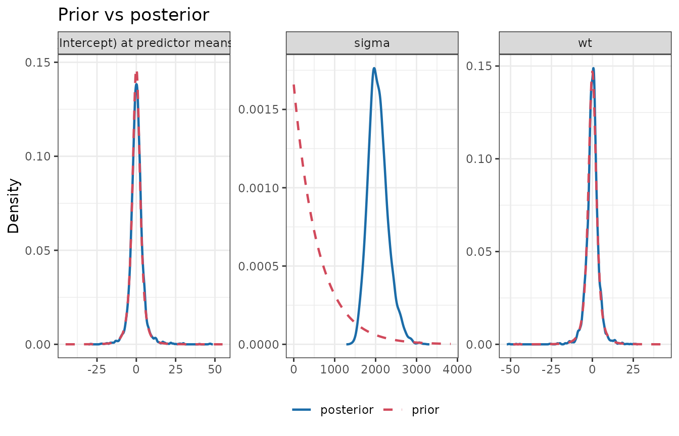
The MCMC diagnostics do not flag this, because the chains mix perfectly well around the wrong answer:
attr(fit_mpg100, "bmb_convergence")$converged
#> [1] TRUE
Two checks catch it. Before fitting, a prior predictive check shows
that these priors expect outcomes centred on zero, far from any
plausible value of mpg * 100:
prior_predictive_check(d, mpg100 ~ wt, prior_config = fixed,
                       plausible_range = c(500, 5000), refresh = 0)
#> <bmb_prior_check> 200 simulated data sets of 32 observations (gaussian family)
#>   Observed outcome range     : [1040, 3390]
#>   Prior predictive quantiles : 1%: -2320 | 5%: -1175 | 50%: 2.063 | 95%: 1241 | 99%: 2446
#>   Mean of simulated data (5%, 50%, 95%): -148.7, -0.6828, 182.7
#>   Share of simulated values outside plausible range [500, 5000]: 85.0%
#>   ! More than 5% of prior predictive values are implausible: consider tighter
#>     or better-located priors.
After fitting, prior_sensitivity() shows that the
posterior is dominated by the prior. The posterior has found a
self-consistent but wrong explanation: with a huge residual SD the data
carry almost no information about the slope, so the local diagnosis is
“weak likelihood”, and the slope’s posterior contraction is small
despite 32 observations with a strong relationship.
s <- prior_sensitivity(fit_mpg100)$summary
s[, c("variable", "mean", "contraction", "diagnosis")]
#>                variable         mean contraction         diagnosis
#> (Intercept) (Intercept) 2.517843e-01 -0.01856442   weak likelihood
#> wt                   wt 6.088883e-02  0.12572857   weak likelihood
#> sigma             sigma 2.061119e+03  0.83814473 informative prior
Power-scaling diagnostics are local: they describe the posterior you obtained, not the one you should have obtained. That is why the prior predictive check, which is a global check, comes first.
Four ways to get the scale right
-
Standardise outcome and predictors, then use
unit-scale priors such as
normal(0, 1). Simple and transparent, but coefficients must be back-transformed for interpretation. -
Autoscale.
prior_spec(..., autoscale = TRUE)lets rstanarm rescale the prior by the standard deviations of the outcome and predictors (Gelman et al., 2008). Components you leaveNULLinprior_config()use rstanarm’s autoscaled defaults. - Use substantive knowledge in the natural units, as in the Get started vignette.
-
Derive priors from data defensibly with
empirical_bayes_priors()(see the Data-informed priors article).
With the (autoscaled) defaults, the two fits agree up to the change of units:
fit_default <- fit_model_with_prior(d, mpg100 ~ wt, refresh = 0)
coef(fit_default)["wt"] / coef(fit_mpg)["wt"]
#>       wt
#> 102.2612
rstanarm::prior_summary() shows what autoscaling
did:
rstanarm::prior_summary(fit_default)
#> Priors for model 'fit_default'
#> ------
#> Intercept (after predictors centered)
#>   Specified prior:
#>     ~ normal(location = 2009, scale = 2.5)
#>   Adjusted prior:
#>     ~ normal(location = 2009, scale = 1507)
#>
#> Coefficients
#>   Specified prior:
#>     ~ normal(location = 0, scale = 2.5)
#>   Adjusted prior:
#>     ~ normal(location = 0, scale = 1540)
#>
#> Auxiliary (sigma)
#>   Specified prior:
#>     ~ exponential(rate = 1)
#>   Adjusted prior:
#>     ~ exponential(rate = 0.0017)
#> ------
#> See help('prior_summary.stanreg') for more details
Prior predictive checks
A prior predictive check simulates outcomes from the priors alone (the likelihood is switched off) and asks whether they look like data that could plausibly have been observed (Gabry et al., 2019). It shows what a set of priors implies in the units of the outcome.
A continuous outcome
data(kidiq, package = "rstanarm")
pc_default <- prior_predictive_check(kidiq, kid_score ~ mom_iq + mom_hs,
                                     plausible_range = c(0, 200), refresh = 0)
pc_default
#> <bmb_prior_check> 200 simulated data sets of 434 observations (gaussian family)
#>   Observed outcome range     : [20, 144]
#>   Prior predictive quantiles : 1%: -164.7 | 5%: -74.91 | 50%: 85.42 | 95%: 245.4 | 99%: 341
#>   Mean of simulated data (5%, 50%, 95%): 11.48, 84.37, 166.5
#>   Share of simulated values outside plausible range [0, 200]: 26.8%
#>   ! More than 5% of prior predictive values are implausible: consider tighter
#>     or better-located priors.
rstanarm’s defaults are deliberately weak: 27% of simulated test scores are negative or above 200. That is often acceptable (weak priors let the data speak), but the check makes the trade-off visible. Priors based on what test scores can look like (see the Get started vignette) keep the simulations in a sensible range.
plot(pc_default)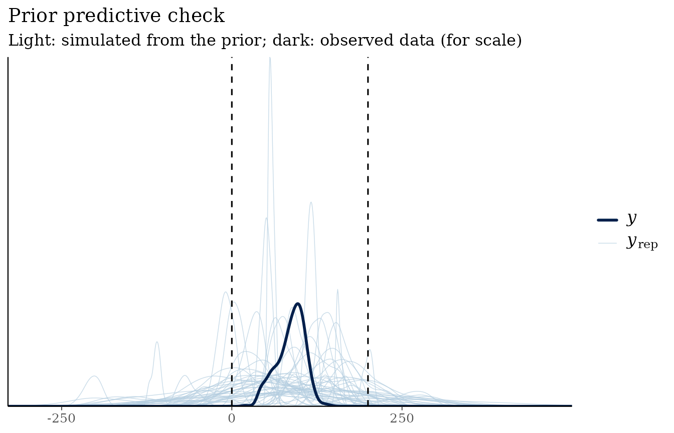
Logistic regression: “non-informative” priors are informative
For binary outcomes, wide priors on the logit scale are a classic
trap. The wells data (Gelman & Hill, 2007) record
whether households in Bangladesh switched away from an unsafe well.
Consider three sets of priors for a model with three predictors:
data(wells, package = "rstanarm")
wells$dist100 <- wells$dist / 100
f <- switch ~ dist100 + arsenic + educ

wide <- prior_config(intercept = prior_spec("normal", 0, 10),
                     slope     = prior_spec("normal", 0, 10))
narrow <- prior_config(slope = prior_spec("normal", 0, 0.5, autoscale = TRUE))

checks <- list(
  "normal(0, 10)"              = prior_predictive_check(wells, f, binomial(), wide, refresh = 0),
  "rstanarm default"           = prior_predictive_check(wells, f, binomial(), NULL, refresh = 0),
  "normal(0, 0.5), autoscaled" = prior_predictive_check(wells, f, binomial(), narrow, refresh = 0)
)
sapply(checks, function(x) x$summary$share_extreme)
#>              normal(0, 10)           rstanarm default
#>                  0.9062070                  0.4960762
#> normal(0, 0.5), autoscaled
#>                  0.2191772
The numbers are the share of prior predictive success probabilities
below 5% or above 95%. The “vague” normal(0, 10) prior
makes 91% of households’ decisions a foregone conclusion. The weakly
informative default still does this for 50%, because the variances of
independent coefficient priors add up on the logit scale as predictors
accumulate (Gelman et al., 2020). Tighter, autoscaled priors bring the
share down to 22%.
plot(checks[["normal(0, 10)"]])
#> Note: in most cases the default test statistic 'mean' is too weak to detect
#> anything of interest.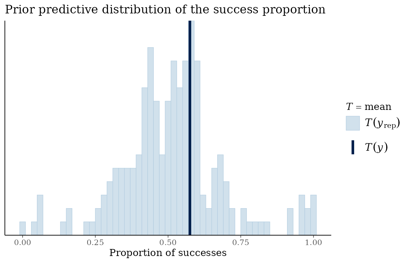
Checklist
- Write priors in the units of your data, or standardise, or autoscale.
- Run
prior_predictive_check()with aplausible_rangeyou can defend. - After fitting, run
prior_sensitivity(): aprior-data conflictor a smallcontractiontells you the prior is doing more work than you may have intended.
References
Gabry, J., Simpson, D., Vehtari, A., Betancourt, M., & Gelman, A. (2019). Visualization in Bayesian workflow. JRSS A, 182(2), 389–402. https://doi.org/10.1111/rssa.12378
Gelman, A., & Hill, J. (2007). Data Analysis Using Regression and Multilevel/Hierarchical Models. Cambridge University Press. https://doi.org/10.1017/CBO9780511790942
Gelman, A., Jakulin, A., Pittau, M. G., & Su, Y.-S. (2008). A weakly informative default prior distribution for logistic and other regression models. The Annals of Applied Statistics, 2(4), 1360–1383. https://doi.org/10.1214/08-AOAS191
Gelman, A., Vehtari, A., Simpson, D., et al. (2020). Bayesian workflow. arXiv:2011.01808. https://doi.org/10.48550/arXiv.2011.01808