Plot the dissimilarity distribution behind an area of applicability

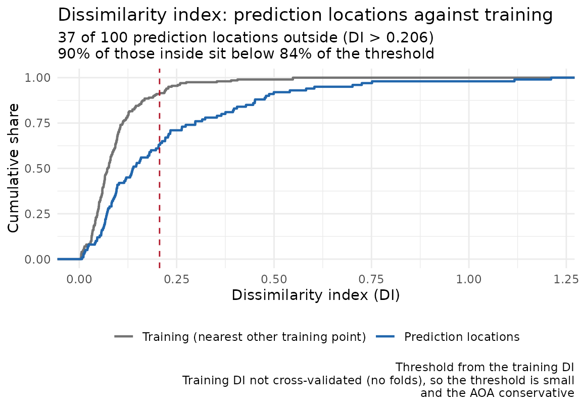
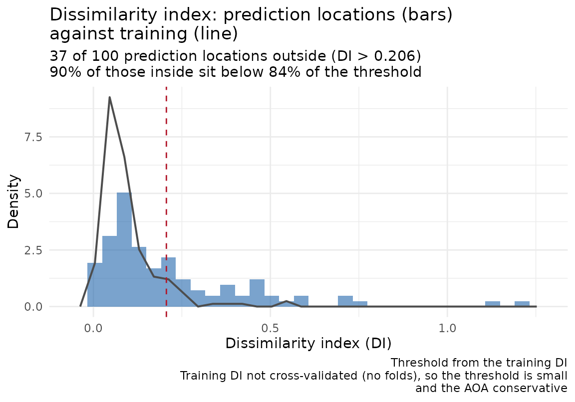
n_outside says how many prediction locations fall outside the area of applicability; it does not say whether the rest sit comfortably inside or crowd against the threshold, nor how far outside the outsiders are. This draws the dissimilarity index of the prediction locations against that of the training data, with the threshold marked, so the prediction set can be read as mostly inside, marginal or largely outside. The training DI is cross-validated over the folds passed to area_of_applicability(), or without them is each training point's distance to its nearest other training point; the legend and the caption say which. The training curve is the reference the threshold was derived from: the threshold is the largest training DI inside an outlier fence, so the curve reaches it exactly when no training value was fenced off and runs past it, by the tail the fence removed, when some were. A prediction location outside on a predictor dropped for having no training variance has DI = Inf: it counts in the prediction curve, which then tops out below 1, and the caption says how many are off the axis. A location with a missing predictor (DI = NA) is neither inside nor outside; it is left out of the curve and the caption counts it.

Usage

# S3 method for class 'aoa'
plot(x, type = c("ecdf", "histogram"), ...)

Arguments

x

An aoa object from area_of_applicability().

type

"ecdf" (default), the two empirical distribution functions on one axis, or "histogram", the prediction DI as bars with the training DI as an outline.

...

Ignored.

Value

A ggplot object.

See also

Other plotting: plot.block_size_sweep(), plot.feature_selection(), plot.gwr_model_selection(), plot.resolution_profile(), plot.sac_range(), plot.spatial_fit(), plot_calibration(), plot_cv_metrics(), plot_folds()

Examples

if (requireNamespace("ggplot2", quietly = TRUE)) {
  library(sf)
  set.seed(2)
  n <- 200
  train <- st_as_sf(
    data.frame(x = 5e5 + runif(n, 0, 1000), y = 5e6 + runif(n, 0, 1000),
               a = rnorm(n), b = rnorm(n)),
    coords = c("x", "y"), crs = 32632)
  train$z <- train$a - train$b + rnorm(n, 0, 0.3)
  # Prediction locations whose predictor `a` drifts beyond the training range.
  new <- st_as_sf(
    data.frame(x = 5e5 + runif(100, 0, 1000), y = 5e6 + runif(100, 0, 1000),
               a = rnorm(100, mean = 2), b = rnorm(100)),
    coords = c("x", "y"), crs = 32632)
  aoa <- area_of_applicability(new, train_sf = train, predictor_vars = c("a", "b"))
  print(plot(aoa))              # the two ECDFs; print() because only a
                                # block's last value is drawn on its own
  plot(aoa, type = "histogram")
}