Choosing a resolution
Justin Chase
30 September 2026
Source:vignettes/resolution.Rmd
resolution.RmdThis article needs two optional packages: gstat, which fits the variogram behind the autocorrelation range, and ggplot2 for the figures. When either is missing the code is shown but not run, and a note at the top says so.
The question
Before point observations can be aggregated into regions, something has to decide how many regions. Twenty cells over a county smooth away most of the variation you came to measure. Two thousand give you cells holding one observation each, where the standard errors are undefined and every cell mean is one number pretending to be an average.
Administrative boundaries settle this by fiat: you get the census tracts that exist. Drawing the regions yourself removes the fiat and leaves the decision with you, and the number propagates into the variance of the cell means, the design effect, and the size of the blocks a spatial cross-validation holds out.
Three functions answer the question, in increasing order of how much
they tell you. determine_optimal_levels() reads an elbow
off the coordinates alone and runs on the hard dependencies; it is the
quick answer and the one build_tessellation() accepts
directly. resolution_profile() scores every cell count on a
ladder against four criteria at once and needs gstat for two of them.
select_resolution() reads one criterion off that profile,
and summary() on the profile reads all four side by side.
If the cells will feed a model, the profile is the one to use. If you
need a count now and the data are all you have, the elbow is defensible
when the points cluster, and this article says where it falls short. On
points spread evenly there is no elbow to read, and both functions say
so: the profile leaves its elbow column empty, and
determine_optimal_levels() warns that the count it still
returns was chosen by the ends of its ladder, not by the data.
The argument that says “how many” is spelled differently by the
function it belongs to: max_levels bounds the elbow’s
ladder, n_levels sets the profile’s,
approx_n_cells and target_cells are what the
grid builders take, and n is what
get_voronoi_seeds() takes. Each of the last three accepts
the object the first two return.
A fixture with known structure
A simulated exponential field, so the structure is known before
anything is fitted. The covariance parameter a = 100 gives
an effective range of 300 units across a 1000-unit square, and
sd = 1 adds a nugget large enough to matter later.
The short answer
determine_optimal_levels() returns a few candidate cell
counts, best first.
lv <- determine_optimal_levels(pts, max_levels = 40)
lv
## [1] 7 6 8This fixture’s points are uniform, so their within-cluster sum of
squares falls like c / k all the way down and bends nowhere
of its own. The call warns that it found no elbow and that
max_levels chose lv: a larger
max_levels would give a larger answer. Read an elbow only
off points that cluster; here the profile below is the better guide.
lv[1] is what get_voronoi_seeds() takes as
n, and what build_tessellation() takes as
approx_n_cells for its "hex" and
"square" methods. Voronoi has no cell count to set: it
grows one cell per point you hand it, which is why the count is set when
you place the seeds rather than when you tessellate them. The last
section shows the two calls in order.
Two things to know about this function before you rely on it. Its
criterion = "morans_i" and
criterion = "combined" settings need both
response_var and predictor_vars; give it only
a response and it warns and falls back to "geometric". And
its ladder runs from 1 to max_levels with no lower bound
from the spatial correlation of the data, so it can prefer cells wider
than the field’s own correlation range. The profile below does impose
that bound, which is why the two can disagree.
The profile
resolution_profile() fits every level on a ladder and
reports what each one costs, so you can see the shape of the trade-off
before picking a point on it. Levels are spaced logarithmically, because
cell diameter falls as
.
prof <- resolution_profile(pts, response_var = "z", n_levels = 16)
prof
## Resolution profile: 16 levels on 500 points
## ladder : 10 to 55 cells (floor 10 from range 314, ceiling 55 from min_cell_n = 9)
## variogram : nugget 0.877, partial sill 1.29, range 314
## scored on : response; 25 k-means++ restarts per level; WSS rises at 0 step(s)
## elbow : none; the WSS curve falls as it does with no cluster structure
##
## levels wss wss_spread elbow cell_n_min cell_n_median cell_diam_median rss
## 10 7850000 0.1510 NA 38 48.0 248.0 914
## 11 6960000 0.0965 NA 31 45.0 233.0 900
## 13 5850000 0.0578 NA 27 40.0 214.0 865
## 14 5500000 0.0810 NA 26 33.0 209.0 862
## 16 4750000 0.0864 NA 24 29.5 194.0 850
## 18 4220000 0.0694 NA 19 27.5 179.0 862
## 20 3750000 0.0666 NA 15 25.0 174.0 793
## 22 3310000 0.1100 NA 15 22.5 163.0 812
## 25 2780000 0.1210 NA 12 20.0 148.0 798
## 28 2390000 0.1380 NA 12 17.0 139.0 778
## 31 2180000 0.1060 NA 9 16.0 130.0 722
## 35 1870000 0.1670 NA 7 14.0 121.0 695
## 39 1650000 0.1310 NA 6 13.0 115.0 686
## 44 1440000 0.0832 NA 6 11.0 107.0 648
## 49 1260000 0.0984 NA 6 10.0 100.0 633
## 55 1110000 0.1280 NA 4 9.0 91.8 638
## cp moran_i moran_z reliability
## 1.86 -0.10600 0.1250 0.811
## 1.84 -0.03160 1.3000 0.806
## 1.78 -0.03700 0.7000 0.798
## 1.77 -0.05140 0.3770 0.793
## 1.76 -0.00625 0.8350 0.785
## 1.79 -0.02540 0.4610 0.777
## 1.66 -0.05660 -0.0528 0.769
## 1.70 0.01360 0.8210 0.761
## 1.68 0.01050 0.7030 0.750
## 1.65 0.00177 0.5310 0.739
## 1.55 0.03950 1.0200 0.729
## 1.51 0.07480 1.5100 0.716
## 1.51 0.02900 0.8280 0.704
## 1.45 0.07390 1.5300 0.689
## 1.44 0.12300 2.3500 0.675
## 1.47 0.18600 3.4400 0.660One row per level. cell_n_median and
cell_diam_median are usually the first two columns worth
reading: how many points a typical cell holds, and how big it is in CRS
units. cell_diam_median is twice the median
root-mean-square distance of a cell’s points from its centre, about 0.8
of the side of a square cell of the same area, so compare it against
something you already know about your own data, such as the spacing of a
sampling grid or the size of a field, with that factor in mind.
The four criteria
| criterion | measures | needs | direction |
|---|---|---|---|
elbow |
how far the log of the within-cluster sum of squares sags below a
power law (the straight log-log line from one cell to the last level);
NA at every level when the points have no cluster
structure |
coordinates only | larger |
cp |
Mallows’ of the piecewise-constant approximation of the response by cell means | a response, and a variogram for the nugget | smaller |
moran_z |
spatial structure surviving in the residuals of the cell means | a response | nearer zero |
reliability |
the share of the spread in the cell means that is signal, not sampling noise | a variogram | larger |
elbow sees the coordinates and knows nothing about what
you measured. cp and reliability split the
practical question in half: how well the cells represent the field, and
whether the cell values can be told apart from noise.
moran_z is the diagnostic, and a large deviate says the
cells are still leaving spatial pattern on the table.
plot(prof)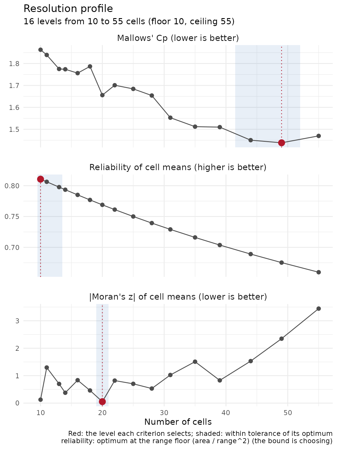
Two behaviours are worth knowing before reading the numbers.
cp needs a nugget to have an interior
optimum. On a smooth field the piecewise-constant approximation
keeps improving as cells shrink, the penalty is too small to stop it,
and the minimum lands wherever min_cell_n stops the ladder.
The support ceiling is then doing the choosing, and
select_resolution() flags it. This fixture has a fitted
nugget of 0.88 against a partial sill of 1.29, which is why
cp turns around inside the ladder here.
reliability rises as cells get larger,
because bigger cells hold more points and average away more noise. Its
optimum can therefore sit on the coarse end of whatever the ladder
allows, which makes the answer a bound on the analysis. The next section
is about spotting that.
Choosing, and the flat region
select_resolution() picks the level a criterion prefers
and reports the band around it.
sel <- select_resolution(prof, criterion = "reliability")
sel
## Resolution by reliability: 10 cells
## flat region : 10 to 13 (3 of 16 levels)
## note : the optimum is the range floor (area / range^2); the bound is
## choosing, not the criterion. Fewer cells would be wider than
## the range and average over more than one patch of the field.sel$best is the optimum and sel$flat is
every level within tol of it. Quote the band when you write
the analysis up. tol is relative to the optimum’s value for
cp and reliability, and relative to the
criterion’s range for elbow and moran_z, whose
optima can be zero.
Two flags say when a bound chose instead of the criterion:
c(at_floor = sel$at_floor, at_ceiling = sel$at_ceiling)## at_floor at_ceiling
## TRUE FALSEat_floor is TRUE here. Reliability wanted
to keep going coarser and the correlation-range floor stopped it, so
read the answer as at most this fine and take the number as a
bound on the analysis, not as an optimum. The floor is a fact about the
data, so the fix is a different question, not a different
tol.
Criteria can prefer different levels while agreeing on a region.
summary() on the profile reads all four at once, and closes
with the levels that every band contains:
summary(prof)## Resolution picks: 3 criteria over 16 levels (10 to 55 cells)
##
## criterion best flat region levels in band
## cp 49 44 to 49 2
## reliability 10 10 to 13 3
## moran_z 20 20 1
##
## reliability: the optimum is the range floor (area / range^2).
## There the bound is choosing, not the criterion.
##
## picks span 10 to 49 cells (4.9x)
## no level is in every flat region: the criteria disagree over the
## whole ladder. plot() draws the curves they were read from.A band is a set of levels, not an interval, because the criterion
curves are not monotone: a band that skips a rung prints as a
comma-separated list, while a solid run of 2 rungs prints as a range, as
cp does with 44 to 49. Where the bands overlap
you have a defensible set of levels, and the last line names it;
attr(summary(prof), "common") returns the same levels for
use in code, and attr(summary(prof), "bands") each
criterion’s region in full. Where they do not overlap, the criteria are
answering different questions and you have to say which one your
analysis needs. An empty intersection is a result: it says this field
has no single resolution that satisfies every way of asking.
The table is not a decision procedure, and nothing in the package will pick for you. Cross-validating a model at each suggested level is affordable, but it does not settle the question either: on a simulated field the level that won on cross-validated moved with the fold seed, and the coarsest grid won most often because its score had the widest spread, not because it was better.
What the ladder can support
The ladder runs between two bounds the data impose, both recorded on the profile.
## List of 11
##  $ floor       : int 10
##  $ ceiling     : int 55
##  $ ceiling_from: chr "min_cell_n"
##  $ supported   : logi TRUE
##  $ area        : num 976371
##  $ range       : num 314
##  $ n           : int 500
##  $ n_sample    : int 500
##  $ n_distinct  : int 500
##  $ min_cell_n  : int 9
##  $ range_floor : logi TRUE
The ceiling is floor(n / min_cell_n), or the number of
distinct locations when that is smaller (one short of it when no
location repeats); ceiling_from says which. Past it the
average cell holds too few points to estimate anything from, or k-means
has more centres to place than distinct points. The floor is
ceiling(area / range^2), from the fitted autocorrelation
range: cells wider than the range average over more than one patch of
the field, mixing values the field itself keeps apart.
When the floor exceeds the ceiling, the data cannot support a
tessellation that respects their own correlation structure.
supported is FALSE, a warning says so, and the
ladder still runs from 2 to the ceiling so the cost of each level stays
visible. The usual causes are too few points for the extent, or a
correlation range shorter than the spacing between observations.
Choosing on one half, estimating on the other
Picking the level from the same response you then aggregate is a form
of double-dipping: the cell count was chosen to suit one realisation of
the field. select_on = "split" profiles part of the layer
and hands back the row positions of both parts.
prof_split <- resolution_profile(pts, response_var = "z", n_levels = 16,
                                 select_on = "split")
sp <- attr(prof_split, "split")
sp
## Spatial half-split (block_kfold, seed 123): 251 selection rows, 249 estimation rows
## $selection and $estimation are row positions in the layer as passed.The split is spatially blocked, not random, and records the method and seed that produced it. A random half would put neighbours of every selection point in the estimation set, and on an autocorrelated field that leaks the structure you are choosing against. Blocking reduces that leak without removing it: the two halves share a border, and points on either side of it within the correlation range are still correlated, so read the separation as a large improvement on a random half rather than as independence.
Choose from prof_split, then aggregate the rows in
sp$estimation. The cells on the ladder are still drawn on
every point, so the count it picks is a count for the whole layer, and
the ladder is as long as the full profile’s. Only the steps that read
the response (the variogram, cp, moran_z) use
the selection half. The cost is power: those criteria see half the data,
so the profile is noisier and the band wider. The estimation rows also
fill only their own half of the layer: a cell inside the selection half
gets none of them, and a cell across the border between the halves is
estimated from the part of it on the estimation side. Read standard
errors only off cells whose points are all estimation rows.
##     floor   ceiling         n supported
##        16        55       500         1
The floor can differ from the full profile’s, because it comes from the range estimated on the selection half.
Next
Hand the selection to whichever call decides the cell count. For a
Voronoi tessellation that is get_voronoi_seeds(). Given the
select_resolution() result itself, it returns the centres
of the partition the profile scored, and a k-means partition is the
Voronoi partition of its centres, so the cells built on those seeds are
the cells the criteria judged; the bare count sel$best
would run a new k-means, whose cells are not.
build_tessellation() then works on the seeds:
bnd   <- clip_target_for(pts, expand = 0.02, quiet = TRUE)
seeds <- get_voronoi_seeds(boundary = bnd, method = "kmeans", n = sel,
                           sample_points = pts)
cells <- build_tessellation(seeds, boundary = bnd, method = "voronoi",
                            quiet = TRUE)
nrow(cells$cells)
## [1] 10For a lattice the count goes to build_tessellation()
itself, and the points go in directly:
hex <- build_tessellation(pts, boundary = bnd, method = "hex",
                          approx_n_cells = sel$best, quiet = TRUE)
nrow(hex$cells)
## [1] 18The hex count overshoots the request: the target is adjusted for
packing density and then clipped to an irregular boundary, so
approx_n_cells is approximate in both directions. The
seeded Voronoi hits the number exactly, because the seeds are the
cells.
Passing approx_n_cells with
method = "voronoi" warns and is ignored. Without the
seeding step you get one cell per observation, which is a
nearest-neighbour interpolation rather than a resolution.
vignette("spatialkit_nc_demo") runs the whole pipeline
on real boundaries. ?resolution_profile documents how each
criterion behaved on simulated fields, with the references;
?determine_optimal_levels covers the k-means++ restart
budget and the nine-cell floor below which the model-aware criteria
carry no information.