spatialkit draws analysis regions, which it calls cells, from where your observations are, instead of borrowing boundaries drawn for other purposes, and summarises point data onto them with a count, a standard error and a pooled value for every cell. It then scores regression models on cross-validation folds that hold out whole blocks of space, and marks where a fitted map extrapolates.
The problem this solves
You have observations at points and need values over areas. The usual move is to borrow boundaries that already exist: ZIP code areas, census tracts, counties, sales territories. They were drawn for mail delivery, enumeration or politics, so part of any answer aggregated onto them comes from the partition. This is the modifiable areal unit problem: the same observations, aggregated under different boundaries, can give different conclusions.
spatialkit draws the cells from the data, in three steps:
- Pick a cell count.
resolution_profile()andselect_resolution()set it from a size of 4.5 observations per cell by default, and report the leave-one-out error of the cell values. Given a ladder of counts, the profile scores each one against the spatial structure of the observations. - Place the cells.
get_voronoi_seeds()places seeds by density-weighted k-means, so cells are small where observations are dense, andbuild_tessellation()grows Voronoi cells from them (or lays hex or square cells, or Delaunay triangles), clipped to your study area.build_tessellation()numbers the cells from their geometry, so the same seeds in a different row order give the same cell IDs. - Summarise.
summarize_by_cell()gives each cell a count, a mean with its standard error, and a pooled value: the cell’s mean pulled toward the mean of the observations in the 8 nearest cells (nearest by the centroid of their observations). When the cell means stand in for a population mean, it can correct the standard errors for autocorrelation within the cells, which on a correlated field can double them or more.
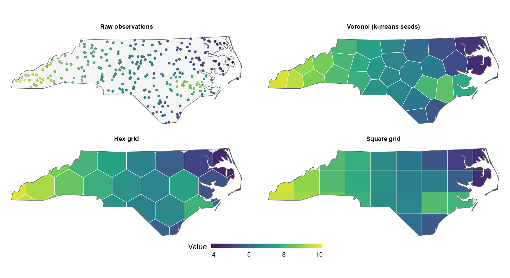
The first figure shows a simulated field on 280 random sites in North Carolina, aggregated onto three kinds of cells, about 30 of each: Voronoi cells from density-weighted seeds, a hex grid and a square grid.
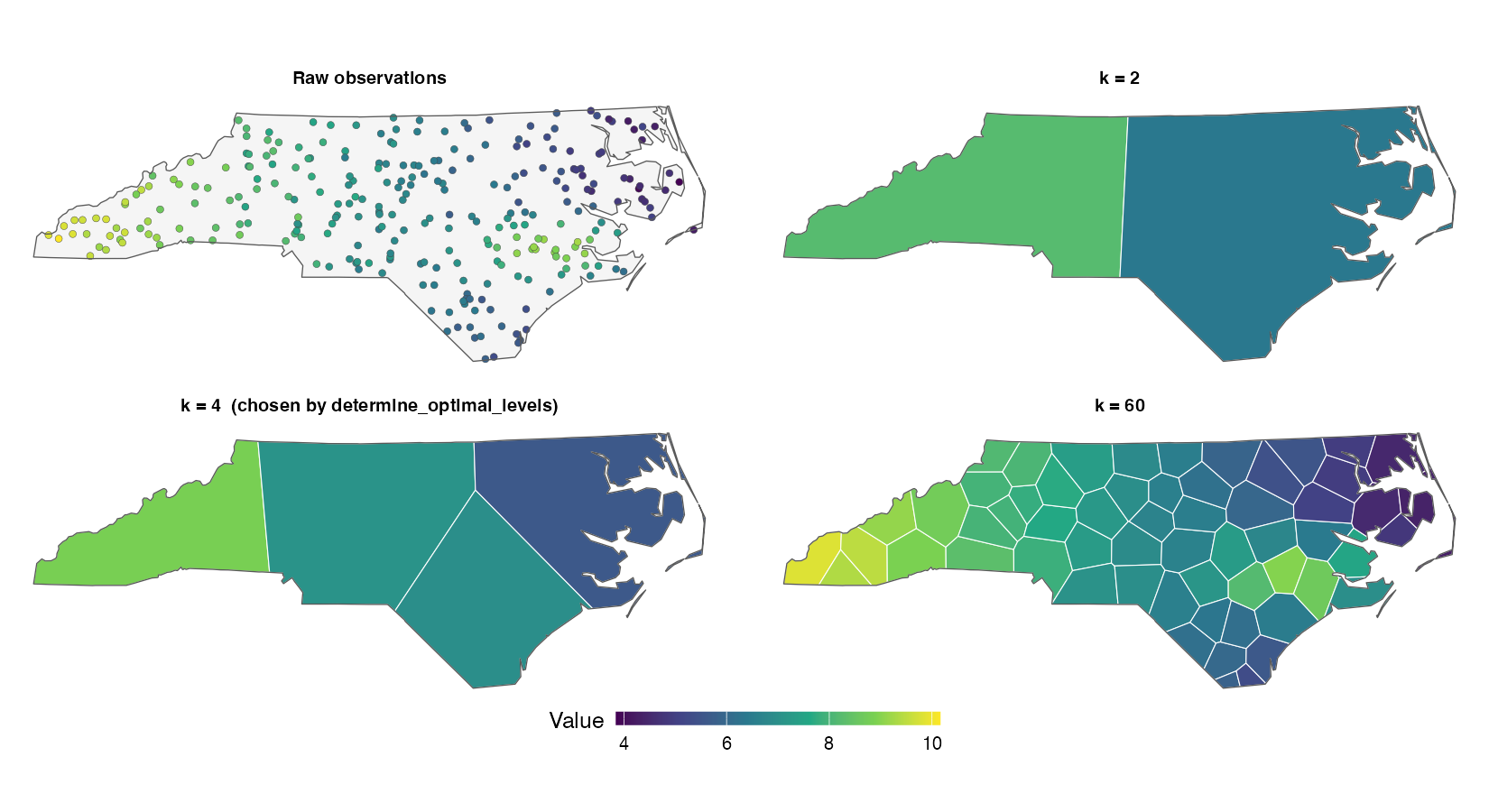
The next figure cuts the same field at three cell counts, each cell showing its pooled value. resolution_profile() scores each count by the leave-one-out error of the pooled values at that count. The error is 0.33 at 12 cells, 0.18 at 62 cells (the count the default size of 4.5 observations per cell gives) and 0.18 at 140 cells (two per cell). The 12 cells blur the hotspot in the east. At 140 cells the error is within one standard error of the default’s. vignette("resolution") covers how the count is chosen.
The second half of the package tests the result. Three model backends (random forest, GWR and a Bayesian GP) sit behind one spatial_fit class, so they can be scored on the same folds. Cross-validation holds out whole blocks, of a grid by default, which can be sized from the data’s own autocorrelation range or matched to the locations a map will predict at. An area-of-applicability estimate marks where the resulting score applies. All of it is built on sf, and each function that measures a distance moves a lon/lat layer into a projected CRS first.
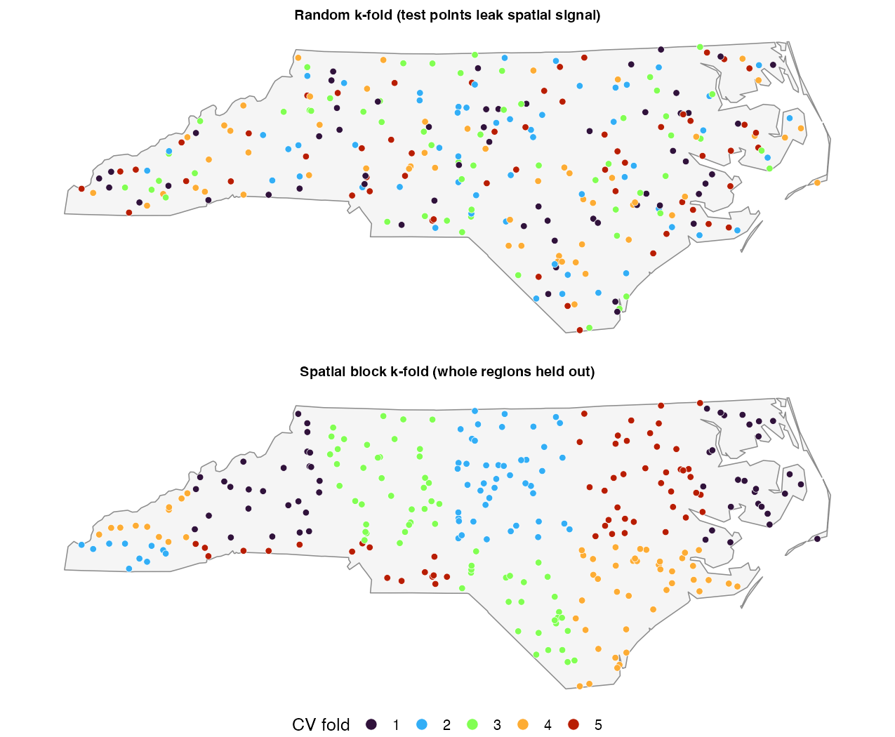
Random folds put a test point’s neighbours in the training set, so a model that can memorise location is scored on points it has nearly seen. Block folds hold out whole blocks instead; the quick start below shows the difference in RMSE.
Scope
-
Regression, with one exception.
fit_rf_model()andfit_gwr_model()fit a numeric response and refuse a logical, factor or character one;fit_gwr_model()also refuses an integer-coded two-valued response and points toGWmodel::ggwr.basic(). The exception isfit_bayesian_spatial_model(), which also fits a binary response underbrms::bernoulli(), and a factor or character response underbrms::categorical()or an ordinal family.cv_bayes()refuses the categorical and ordinal families, because it scores one predicted number per row. -
Vector data only. There is no raster input or output:
predict_surface()returns ansfPOINT layer, which you convert yourself if you need aSpatRaster. The models work on points:prep_model_data()andcoerce_to_points()reduce lines and polygons to points. - No areal or lattice models. Moran’s I here tests residuals for spatial structure. There is no CAR, SAR or spatial-lag fitter.
- No spatio-temporal folds. Every fold scheme is spatial; none holds out time.
Installation
install.packages("spatialkit")The development version installs from GitHub:
# install.packages("remotes")
remotes::install_github("elkronos/gis_modeling_toolkit")sf, dplyr, logger, digest and FNN install with it. Optional packages switch on the model backends, variograms and plots; Get started lists which does what. If you are upgrading from 2.0.0, the changelog lists the defaults that change results and the argument that restores each.
Quick start
A simulated field of 400 observations in a 1,000 m square, with one weak measured predictor w:
library(sf)
library(spatialkit)

set.seed(42)
n  <- 400
xy <- data.frame(x = 5e5 + runif(n, 0, 1000), y = 5e6 + runif(n, 0, 1000))
D  <- as.matrix(dist(xy))
xy$w <- rnorm(n)
# Mostly a smooth spatial field (exponential, effective range 3 x 80 = 240 m),
# with the weak predictor on top.
xy$z <- 0.5 * xy$w +
  as.numeric(t(chol(exp(-D / 80) + diag(1e-8, n))) %*% rnorm(n)) +
  rnorm(n, sd = 0.3)
site <- st_as_sf(xy, coords = c("x", "y"), crs = 32632)
Set the cell count, draw Voronoi cells from the data and summarise onto them:
size <- select_resolution(resolution_profile(site, "z"))
size
#> Resolution by size: 89 cells
#>   size        : 4.5 rows per cell, the default (obs_per_cell); 400 rows / 89 cells = 4.49
#>   cells       : density-weighted k-means++ starts (power 1, 8 neighbours)
#>   estimate    : pooled toward the 8 nearest cells
#>   at this size: 0.0% of the rows are alone in their cell; median own weight 0.78
#>   loo         : 0.912 (one cell for the layer: 1.5)
#>   note        : the count is set by obs_per_cell = 4.5, the default; no
#>                 criterion chose it.

seeds <- get_voronoi_seeds(n = size, sample_points = site)
tess  <- build_tessellation(seeds,
                            boundary = clip_target_for(site, quiet = TRUE),
                            method = "voronoi", quiet = TRUE)
asg   <- assign_features_to_polygons(site, tess$cells,
                                     polygon_id_col = "cell_id")
cells <- summarize_by_cell(asg, "z", id_col = "cell_id", cells_sf = tess$cells)

head(st_drop_geometry(cells)[, c("cell_id", "n", "resp_mean_z", "..se_resp_z",
                                 "..pooled_resp_z")], 4)
#>   cell_id n resp_mean_z ..se_resp_z ..pooled_resp_z
#> 1       1 4   1.3680408   0.3289247       1.0626423
#> 2       2 3  -0.2762594   0.1258383      -0.1086915
#> 3       3 3  -0.9436130   0.5218985      -0.6630103
#> 4       4 5  -1.9008715   0.1581262      -1.4425290
The default size gives 89 cells, each holding between 2 and 10 observations. Each row has a count, the cell mean, its standard error and the pooled value ..pooled_resp_z, the cell’s mean pulled toward its neighbours by a weight that grows with the cell’s count (?summarize_by_cell, “Pooled values”). That standard error is the one for the cell’s own mean when its points are spread through the cell. When the cell means stand in for the population mean, deff = "kish" widens each standard error for the correlation inside the cell; on these cells it multiplies them by 2.2 (median). ?summarize_by_cell says which to use when.
Then score a model. A random forest given the coordinates (include_coords = TRUE) can fit the training surface by memorising location. Score it on random folds and on blocks of at least 250 m, just above the field’s effective range (this needs ranger):
fr <- make_folds(site, k = 5, method = "random_kfold", seed = 1)
fb <- make_folds(site, k = 5, method = "block_kfold", block_size = 250,
                 seed = 1)

random  <- cv_rf(site, "z", "w", folds = fr, include_coords = TRUE)
blocked <- cv_rf(site, "z", "w", folds = fb, include_coords = TRUE)

c(random = random$overall$RMSE, blocked = blocked$overall$RMSE)
#>    random   blocked
#> 0.9790119 1.1227029
On the same 400 observations and the same model, random folds give an RMSE of 0.98 and the blocks, built 332 m wide, give 1.12. The data and the model are the same; the random figure is the error of predicting among the samples, and the blocked one the error of predicting into gaps a block wide. A map’s error depends on where it predicts, and fold_separation() compares the folds’ distances from the training data with the map’s. On real data the range is estimated, by estimate_sac_range() or make_folds(auto_range = TRUE); vignette("spatial-cross-validation") covers that choice.
The pipeline
Steps 1 to 10 link to their section of the reference index, and every step to the article that shows it. ?spatialkit lists the same steps inside R.
Where to go next
The articles, in reading order:
| Article | What it covers | In R |
|---|---|---|
| Get started | Take a layer of points to cells with standard errors, a score from spatial cross-validation and a map that marks where its predictions apply. | vignette("getting-started") |
| Choosing a resolution | Decide how many cells the data support, and pass that count to the tessellation. | vignette("resolution") |
| Building cells and summarising them | Draw the cells, put each observation in one, and report each cell’s value with the right standard error. | vignette("cells") |
| Spatial cross-validation | Choose folds whose score matches the map you will make, size the blocks, and read every part of the result. | vignette("spatial-cross-validation") |
| Fitting and checking models | Pick a backend or write your own, compare backends on the same folds, check the residuals, and map where the predictions apply. | vignette("models") |
| Exporting and reporting results | Write the cells to a file others can join to, and report the numbers that say how far a cell value or a map can be trusted. | vignette("reporting") |
| Worked example: North Carolina | The pipeline on a simulated field over North Carolina, comparing four tessellations, two fold schemes and two backends at cell counts set by hand. | vignette("spatialkit_nc_demo") |
| Troubleshooting and performance | The errors and warnings you are most likely to meet, what each means, and how to handle large layers, parallel folds, caches and the log. | vignette("troubleshooting") |
| Terms used on these pages | Short definitions of the terms the articles and help pages use. | vignette("glossary") |
The numbered scripts in system.file("scripts", package = "spatialkit") run each step on a simulated field; Get started lists them. Report a bug or ask a question on the issue tracker; the contributing guide says what to include.
Citation
citation("spatialkit")This prints the package entry and the papers behind the methods spatialkit implements. Cite the paper as well as the package if you rely on area_of_applicability() (Meyer and Pebesma 2021), make_folds(method = "nndm") (Milà et al. 2022) or make_folds(method = "knndm") (Linnenbrink et al. 2024). Do the same for the model backends you use: the Hilbert space approximation in fit_bayesian_spatial_model() (Riutort-Mayol et al. 2023), permutation importance in fit_rf_model() (Strobl et al. 2007), coordinates as predictors and blocked validation in fit_rf_model() and cv_rf() (Meyer et al. 2019), and GWR, whose kernels and diagnostics follow GWmodel (Lu et al. 2014).
Licence
MIT, © Justin Chase; see LICENSE.md. spatialkit is a personal project, developed independently and not affiliated with or endorsed by any organisation. It contains no confidential, proprietary or non-public information.