spatialkit: Tessellations, Spatial Cross-Validation and Models

Overview

This vignette generates synthetic spatial data over North Carolina and walks through the spatialkit workflow end to end:

Load the boundary and check which optional packages are present
Simulate observations with known structure over it
Build four tessellation types (Voronoi, hex, square, Delaunay)
Assign points to cells, aggregate with summarize_by_cell(), and map the cell means
Estimate the autocorrelation range, build spatial CV folds, and score a model under blocked versus random folds
Fit the models to keep: a random forest, GWR when it is installed, and the two compared on identical folds
Predict onto a surface and mark where that surface is extrapolation

Everything is self-contained — the boundary comes from the nc.shp demo shapefile bundled with sf, so no external files are needed.

Optional backends are checked at the top and every section that needs one is guarded, so this document renders with whatever you happen to have installed. This table always runs, even when the gate below it is shut – it is what says which backend is missing when the code stops producing output:

##        package available                          used_for
## 1      ggplot2      TRUE                         all plots
## 2    patchwork      TRUE     the stacked comparison panels
## 3     geometry      TRUE       true Delaunay triangulation
## 4       ranger      TRUE             random forest backend
## 5        gstat      TRUE variogram / autocorrelation range
## 6 GWmodel + sp      TRUE                       GWR backend

1. Packages and boundary

library(spatialkit)
library(sf)
library(dplyr)
library(ggplot2)

set.seed(42)

We load the North Carolina county boundaries shipped with sf, dissolve them into a single state outline, and project to NAD83 / North Carolina (ftUS) (EPSG:2264) so distances are planar rather than angular. Every distance, bandwidth and block size below is therefore in US survey feet, not metres — projected does not mean metric, and the unit is whatever the CRS says it is:

nc_counties <- st_read(system.file("shape/nc.shp", package = "sf"), quiet = TRUE)
nc_boundary <- nc_counties |>
  st_union() |>
  st_transform(2264) |>
  st_as_sf()

2. Synthetic observations

300 points inside the state boundary with two predictors and a spatially varying response:

elevation — gradient increasing west to east, plus noise
pop_density — decays with distance from two fake “cities”
y — driven by the two predictors plus a spatial field neither of them explains. That last term is deliberate: it is the unmodelled spatial structure that makes random cross-validation optimistic, and it is what section 5 measures.

n_points <- 300

pts_raw    <- st_sample(nc_boundary, size = n_points, type = "random")
pts_coords <- st_coordinates(pts_raw)
x_coords   <- pts_coords[, 1]
y_coords   <- pts_coords[, 2]

elevation <- scale(x_coords)[, 1] * 500 + rnorm(n_points, 3000, 400)

city1 <- c(1530000, 550000)   # Charlotte-ish in EPSG:2264
city2 <- c(2150000, 750000)   # Raleigh-ish
dist_to_city <- pmin(
  sqrt((x_coords - city1[1])^2 + (y_coords - city1[2])^2),
  sqrt((x_coords - city2[1])^2 + (y_coords - city2[2])^2)
)
pop_density <- pmax(exp(-dist_to_city / 400000) * 5000 + rnorm(n_points, 200, 100), 10)

spatial_field <- 20 * sin(x_coords / 250000) * cos(y_coords / 250000)

y_response <- 50 +
  0.01  * elevation +
  0.005 * pop_density +
  spatial_field +
  rnorm(n_points, 0, 5)

points_sf <- st_sf(
  y           = y_response,
  elevation   = elevation,
  pop_density = pop_density,
  geometry    = pts_raw
)

ggplot() +
  geom_sf(data = nc_boundary, fill = "grey95", colour = "black") +
  geom_sf(data = points_sf, aes(colour = y), size = 1.1) +
  scale_colour_viridis_c(name = "Response (y)") +
  theme_void() +
  ggtitle("Raw observation points, North Carolina")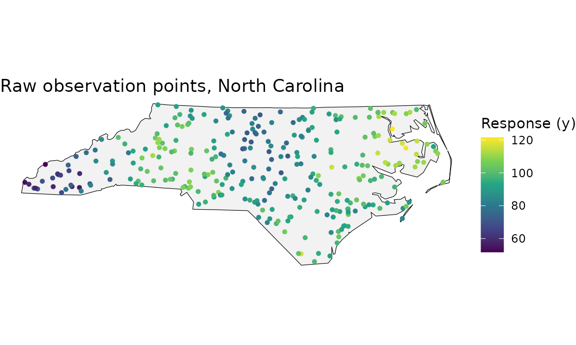

Three hundred simulated observation points scattered across North Carolina, coloured by response value. Lower values cluster in the west and higher values along the eastern coast.

3. Four tessellations

3a. Voronoi from ~40 k-means seeds

Voronoi cells are built around seed points, not the observations themselves. Seeding one cell per observation would give 300 cells each containing a single point — a nearest-neighbour interpolation rather than an aggregation, with no within-cell variation to compute a standard error from. get_voronoi_seeds() clusters the observations first, so cell size follows sampling density.

seeds <- get_voronoi_seeds(
  boundary      = nc_boundary,
  sample_points = points_sf,
  method        = "kmeans",
  n             = 40
)

tess_voronoi <- build_tessellation(
  seeds, boundary = nc_boundary,
  method = "voronoi", clip = TRUE, quiet = TRUE
)

3b and 3c. Hex and square grids (~50 cells)

tess_hex <- build_tessellation(
  points_sf, boundary = nc_boundary,
  method = "hex", approx_n_cells = 50, clip = TRUE, quiet = TRUE
)

tess_square <- build_tessellation(
  points_sf, boundary = nc_boundary,
  method = "square", approx_n_cells = 50, clip = TRUE, quiet = TRUE
)

All four methods return cells carrying a cell_id column; the grid methods keep poly_id alongside it, holding the same values.

names(tess_hex$cells)

## [1] "poly_id"  "geometry" "cell_id"

3d. Delaunay triangles

method = "triangles" uses geometry::delaunayn() when geometry is installed. Without it, it does not error — it falls back to sf::st_triangulate() (GEOS) on the point set and logs a warning. That is still the Delaunay triangulation of the input points; only the resolution of degenerate configurations can differ. Because the two paths are not identical, this section is guarded on geometry rather than on the call succeeding:

tess_tri <- build_tessellation(
  points_sf, boundary = nc_boundary,
  method = "triangles", clip = TRUE, quiet = TRUE
)
nrow(tess_tri$cells)

## [1] 586

cat(sprintf(
  "Voronoi: %d | Hex: %d | Square: %d | Triangles: %s\n",
  nrow(tess_voronoi$cells),
  nrow(tess_hex$cells),
  nrow(tess_square$cells),
  if (has_geom) nrow(tess_tri$cells) else "skipped (install 'geometry')"
))

## Voronoi: 40 | Hex: 49 | Square: 45 | Triangles: 586

# has_geom is requireNamespace("geometry", quietly = TRUE), set in the
# hidden setup chunk with the other availability flags the table above shows.

4. Cell-level aggregation with `summarize_by_cell()`

assign_features_to_polygons() joins points to cells; summarize_by_cell() does the aggregation — means, standard deviations and standard errors for the response and every predictor, plus n and cell_weight. There is no need to write the group_by()/summarise() by hand, and doing so loses the design-effect machinery below.

assigned <- assign_features_to_polygons(points_sf, tess_voronoi$cells,
                                        polygon_id_col = "cell_id")

cell_stats <- summarize_by_cell(
  assigned,
  response_var   = "y",
  predictor_vars = c("elevation", "pop_density"),
  id_col         = "cell_id"
)

head(as.data.frame(cell_stats)[, c("cell_id", "n", "resp_mean_y",
                                   "..sd_resp_y", "..se_resp_y")])

##   cell_id n resp_mean_y ..sd_resp_y ..se_resp_y
## 1       1 6    62.89141    7.074136    2.888004
## 2       2 7    63.36230    7.516155    2.840840
## 3       3 5    67.11282    8.521317    3.810849
## 4       4 5    70.34951   12.427812    5.557886
## 5       5 5    79.61205    5.327447    2.382507
## 6       6 4    84.14516    7.886035    3.943018

The ..se_* columns are IID standard errors at the default deff = 1. That is the right standard error for each cell’s own mean, the value a choropleth shows, when the points are spread through the cell. As a standard error for the population (grand) mean it is anticonservative when points inside a cell are spatially correlated. For that population-level use, deff = "kish" applies Kish’s design-effect correction from an estimated intra-class correlation, and attr(., "deff_applied") records what was used:

cell_kish <- summarize_by_cell(
  assigned,
  response_var   = "y",
  predictor_vars = c("elevation", "pop_density"),
  id_col         = "cell_id",
  deff           = "kish"
)

deff <- attr(cell_kish, "deff_applied")
cat(sprintf("method = %s | ICC(response) = %.3f | median design effect = %.2f\n",
            deff$method, deff$icc_resp, stats::median(deff$deff, na.rm = TRUE)))

## method = kish | ICC(response) = 0.742 | median design effect = 5.45

# Inflation of the response standard error, cell by cell.
summary(cell_kish$`..se_resp_y` / cell_stats$`..se_resp_y`)

##    Min. 1st Qu.  Median    Mean 3rd Qu.    Max. 
##   3.535   4.271   4.595   4.705   5.183   6.193

Choropleths

#' Assign points to cells, summarise, and draw a choropleth.
make_choropleth <- function(tess, boundary, points, title = NULL) {
  cells    <- tess$cells
  assigned <- assign_features_to_polygons(points, cells, polygon_id_col = "cell_id")

  stats_df <- summarize_by_cell(assigned, response_var = "y",
                                id_col = "cell_id")
  cells    <- left_join(cells, as.data.frame(stats_df)[, c("cell_id", "resp_mean_y")],
                        by = "cell_id")

  plot_tessellation_map(
    tessellation_sf = cells,
    boundary        = boundary,
    fill_col        = "resp_mean_y",
    palette         = "viridis",
    tile_alpha      = 0.9,
    outline_col     = "white",
    outline_size    = 0.3,
    boundary_col    = "grey20",
    boundary_size   = 0.8,
    legend_title    = "Mean y",
    title           = title,
    subtitle        = sprintf("%d cells | %d observations",
                              nrow(cells), nrow(points))
  )
}

make_choropleth(tess_voronoi, nc_boundary, points_sf, "Voronoi tessellation")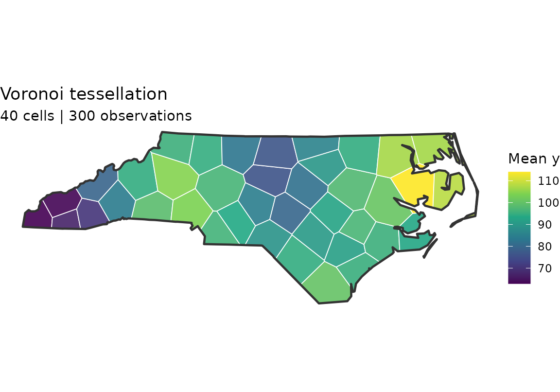

The same response aggregated into forty Voronoi cells over North Carolina. Cell sizes follow the density of the observations, and the west-to-east gradient from low to high values is visible.

Voronoi choropleth

make_choropleth(tess_hex, nc_boundary, points_sf, "Hexagonal grid")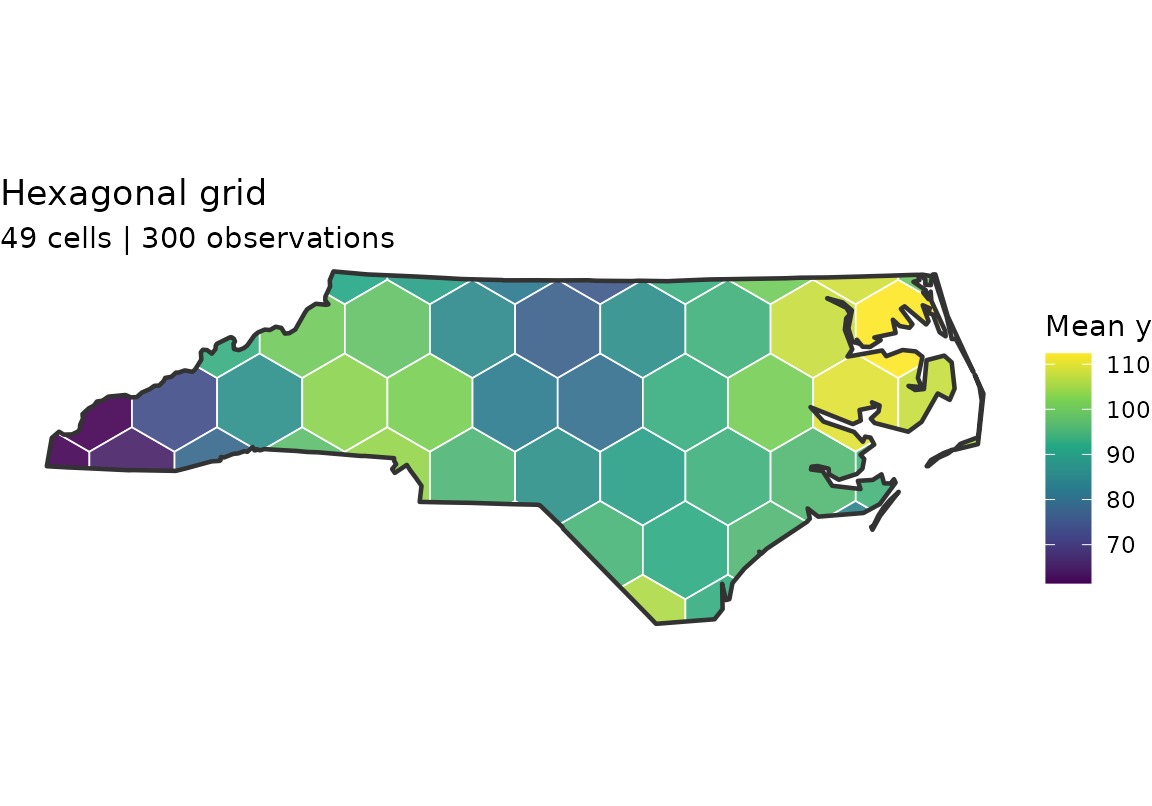

The same response aggregated into a regular hexagonal grid of about fifty equal-area cells, showing the same west-to-east gradient on a fixed geometry rather than one drawn from the data.

Hex grid choropleth

make_choropleth(tess_square, nc_boundary, points_sf, "Square grid")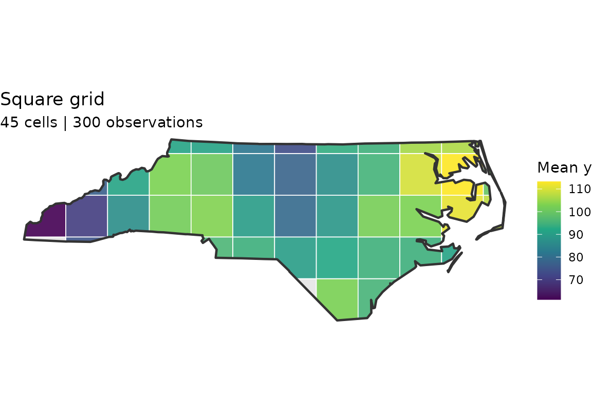

The same response aggregated into a regular square grid of about forty-five cells, showing the same gradient with the axis-aligned artefacts a square grid introduces.

Square grid choropleth

make_choropleth(tess_tri, nc_boundary, points_sf, "Delaunay triangulation")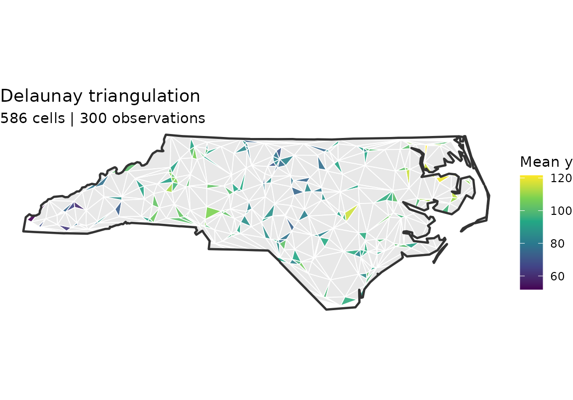

The same response aggregated onto the Delaunay triangulation of the observation points, which produces many small irregular triangles rather than compact cells.

Delaunay choropleth

The three stacked on one shared colour scale. Each map drawn on its own gets its own scale, so a colour in one means a different value in the next; here the limits are set from all three together and patchwork then collects the legends into one, which is what makes reading down the page legitimate.

library(patchwork)

# The cell means of all three, so the colour scale can span them.
cell_means <- function(tess) {
  a <- assign_features_to_polygons(points_sf, tess$cells, polygon_id_col = "cell_id")
  summarize_by_cell(a, response_var = "y", id_col = "cell_id")$resp_mean_y
}
lims <- range(unlist(lapply(list(tess_voronoi, tess_hex, tess_square), cell_means)),
              na.rm = TRUE)

# One line per map instead of a title and a subtitle, and the cell count taken
# from the tessellation rather than typed in.
bare <- function(tess, label) {
  make_choropleth(tess, nc_boundary, points_sf) +
    ggplot2::scale_fill_viridis_c(name = "Mean y", limits = lims) +
    ggplot2::labs(title = sprintf("%s, %d cells", label, nrow(tess$cells)),
                  subtitle = NULL) +
    ggplot2::theme(plot.title = ggplot2::element_text(size = ggplot2::rel(1)))
}

(bare(tess_voronoi, "Voronoi") /
 bare(tess_hex,     "Hex") /
 bare(tess_square,  "Square")) +
  plot_layout(guides = "collect") +
  plot_annotation(title = "Tessellation comparison, cell-level mean response")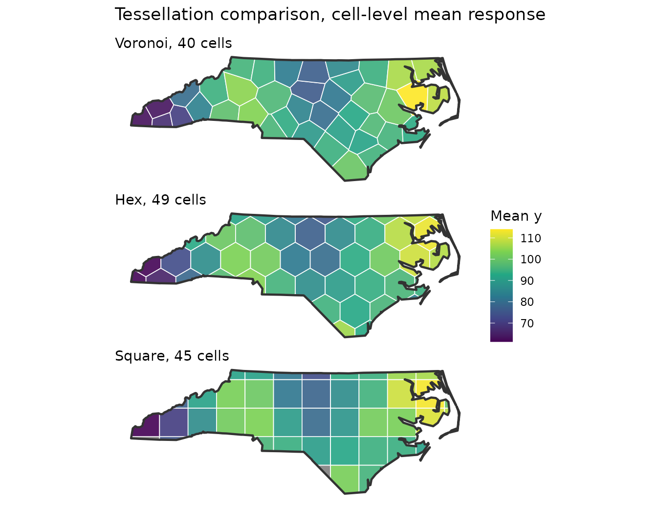

The Voronoi, hexagonal and square maps stacked on one shared colour scale, so the cell values can be compared down the page. All three show the same west-to-east gradient; they differ in how the cell boundaries fall.

All three at a glance

5. Spatial cross-validation

This is the part the rest of the package exists to support.

5a. How far does correlation reach?

estimate_sac_range() fits an omnidirectional variogram and returns the effective range in CRS units — here, US survey feet. It also fits the four principal directions and reports their ranges in the directional attribute (with their largest-over-smallest ratio in anisotropy), but only as a diagnostic: each direction sees about a quarter of the point pairs, the maximum of four such fits is biased upward, and the windows are fixed to the coordinate axes, so nothing built from them is invariant to rotating the layer. The all-pairs fit is the estimate whenever it is usable; the directional maximum stands in for it only when the all-pairs fit fails, and the anisotropy_used attribute is TRUE in that case alone. If you know the field is anisotropic, size blocks from the longest directional range explicitly: max(attr(sac, "directional_fitted"), na.rm = TRUE), after checking attr(sac, "directional_status"), since directional is NA for a direction that ran past the fitted lags, which on such a field is often the long one. It returns NA (still classed sac_range, so it prints as NA) when the empirical variogram never reaches a sill, because an unidentified range must not be used to size blocks.

sac <- estimate_sac_range(points_sf, response_var = "y",
                          predictor_vars = c("elevation", "pop_density"))
sac

## NA 
##   directional: 0 deg = 22475325 (past the fitted lags), 45 deg = 1243020, 90 deg = 1591410 (past the fitted lags), 135 deg = 3346918 (past the fitted lags)
##   in US survey feet of EPSG:2264; variogram of the residuals on predictor_vars (ols)

if (is.na(sac)) {
  cat("no identified range:", attr(sac, "rejected_reason"), "\n")
} else {
  cat(sprintf("range = %.0f ft; anisotropy ratio %.2f; used %s\n",
              as.numeric(sac), attr(sac, "anisotropy"),
              attr(sac, "anisotropy_used")))
}

## no identified range: fitted range exceeds the largest lag fitted

The variogram is attached either way, so plot(sac) draws the curve and lets you judge it rather than trust it (plot(fit, type = "variogram") does the same for a fitted model’s residuals). The distance axis is labelled in the units of the CRS the variogram was fitted in, and when no range was identified the subtitle says why. A rejected range must not be handed to make_folds(auto_range = TRUE), which is why it comes back NA rather than as a long range.

5b. Two fold schemes on the same data

# No range was identified in 5a, so the block size cannot come from the
# variogram.  The field was built as a sine wave with a quarter-wavelength of
# about 390,000 ft, the scale over which it changes sign; 400,000-ft blocks
# hold out whole lobes of it.  cv_block_size_sweep() is the tool for sizing
# blocks by measurement when nothing is known in advance.
folds_random  <- make_folds(points_sf, k = 5, method = "random_kfold", seed = 42)
folds_blocked <- make_folds(points_sf, k = 5, method = "block_kfold",
                            block_size = 400000, seed = 42)

c(random = folds_random$k, blocked = folds_blocked$k,
  blocks = folds_blocked$params$blocks_used)

##  random blocked  blocks 
##       5       5      12

plot_folds() is the fastest way to see whether the blocks actually separate the data or are smaller than the autocorrelation range and therefore leaking:

library(patchwork)
(plot_folds(folds_random,  points_sf, boundary = nc_boundary) /
 plot_folds(folds_blocked, points_sf, boundary = nc_boundary)) +
  plot_layout(guides = "collect")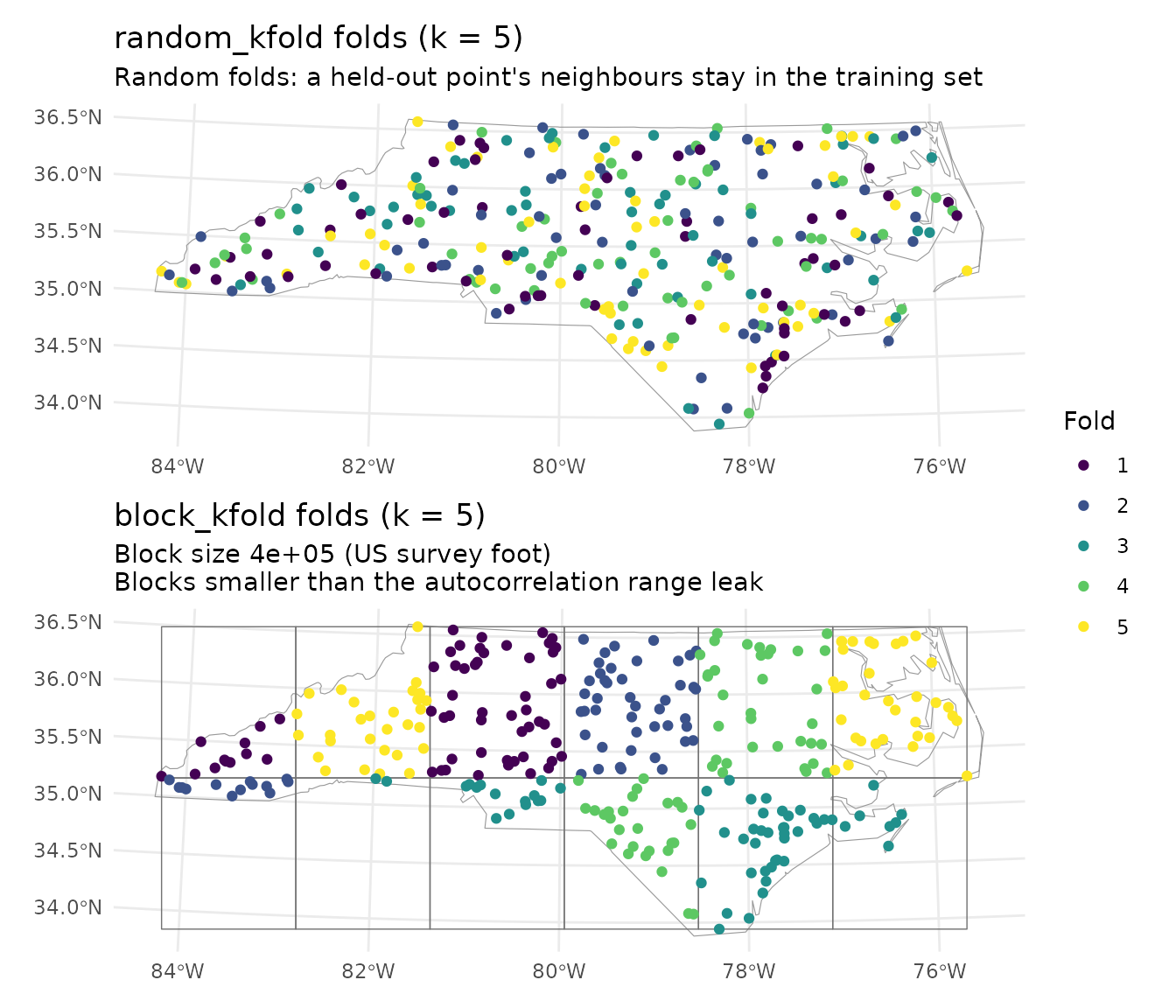

5c. The number the fold scheme changes

fit_rf_model() and cv_rf() need ranger. include_coords = TRUE hands the forest the coordinates, which lets it memorise the training surface — the failure mode the default (FALSE) exists to prevent, and the one random folds cannot see. Scoring the same model on both fold schemes shows the size of the gap:

cv_random  <- cv_rf(points_sf, "y", c("elevation", "pop_density"),
                    folds = folds_random, include_coords = TRUE,
                    num_trees = 300, seed = 1)
cv_blocked <- cv_rf(points_sf, "y", c("elevation", "pop_density"),
                    folds = folds_blocked, include_coords = TRUE,
                    num_trees = 300, seed = 1)

data.frame(
  folds = c("random_kfold", "block_kfold"),
  R2    = c(cv_random$overall$R2,   cv_blocked$overall$R2),
  RMSE  = c(cv_random$overall$RMSE, cv_blocked$overall$RMSE)
)

##          folds        R2     RMSE
## 1 random_kfold 0.7945653 6.089268
## 2  block_kfold 0.6310837 8.997421

Random folds report R² = 0.795; blocked folds report 0.631 on the same fitted model, a drop of 21% of the reported skill.

The blocked estimate is the one to report. The random one describes interpolation between points you already have, which is not the task.

6. Fitting a model

rf_fit <- fit_rf_model(points_sf, response_var = "y",
                       predictor_vars = c("elevation", "pop_density"))
rf_fit

## <Random Forest (ranger)> spatial model fit
##   Formula : y ~ elevation + pop_density
##   n       : 300
##   CRS     : EPSG:2264
##   Trees   : 500 (mtry = 1, min node = 5)
##   Coords as predictors: no
##   Sampling: bootstrap, with replacement (100.0% of rows per tree)
##   OOB RMSE: 9.7284   OOB R^2: 0.4733
##   Importance (permutation): elevation=105.4, pop_density=83.25
## 
##   OOB is a random hold-out and is optimistic under spatial
##   autocorrelation; use cv_rf() for a spatial estimate.

Note that summary() on an rf_fit reports out-of-bag metrics, not in-sample ones — fitted.rf_fit() returns out-of-bag predictions, and the printout says so. A gwr_fit or bayesian_fit reports genuinely in-sample metrics, so the two are not comparable; compare_models_cv() is.

summary(rf_fit)

## Summary of <rf_fit> fit (n = 300)
## 
##   Formula: y ~ elevation + pop_density
## 
##   Out-of-bag metrics (NOT in-sample; see ?fit_rf_model):
##     RMSE    = 9.7284
##     MAE     = 7.8448
##     R^2     = 0.4715
##     SMAPE   = 8.65%

rf_fit$info$importance     # coef() on an rf_fit errors: a forest has no coefficients

##   elevation pop_density 
##   105.35583    83.25089

The two printouts disagree in the third decimal of R² — 0.4733 above, 0.4715 here — while reporting an identical RMSE. Neither is wrong, and neither is a bug. Both read the same out-of-bag predictions; they differ only in the denominator of the variance they compare against. print.rf_fit() echoes ranger’s own r.squared, which is 1 - MSE_oob / var(y) using the unbiased (n − 1) sample variance. summary() recomputes 1 - SS_res / SS_tot from the predictions, where SS_tot = sum((y - mean(y))^2) — an n denominator. The unexplained fraction therefore differs by exactly the factor n / (n − 1), here 300/299, and RMSE, which involves no such comparison, matches to four decimals. If you need a figure comparable across backends, use cv_rf() rather than either.

Residual diagnostics

plot() on any spatial_fit maps the residuals; visible structure means unmodelled spatial autocorrelation. residual_morans_i() puts a number on it.

plot(rf_fit, type = "residuals")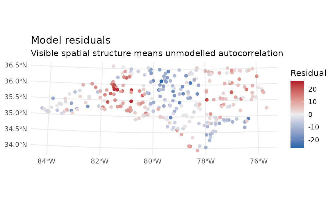

Residuals of the random forest mapped over North Carolina on a red-to-blue scale. Positive residuals cluster in the west and negative ones through the centre, which is the visible spatial structure the model has not captured.

mi <- residual_morans_i(rf_fit)
cat(sprintf("Moran's I = %.4f (z = %.2f, p = %.3g)\n",
            mi$observed, mi$z, mi$p_value))

## Moran's I = 0.5443 (z = 20.12, p = 4.58e-90)

GWR, if `GWmodel` is installed

gwr_fit <- fit_gwr_model(
  data_sf        = points_sf,
  response_var   = "y",
  predictor_vars = c("elevation", "pop_density"),
  adaptive       = TRUE,
  kernel         = "bisquare"
)

gwr_met <- model_metrics(gwr_fit)
# With adaptive = TRUE the bandwidth is a number of nearest neighbours, not a
# distance in feet: each local regression uses the same count of points.
cat(sprintf("Bandwidth: %.0f neighbours | in-sample R2: %.3f | RMSE: %.3f\n",
            gwr_fit$info$bandwidth, gwr_met$R2, gwr_met$RMSE))

## Bandwidth: 42 neighbours | in-sample R2: 0.879 | RMSE: 4.664

The fit raises no collinearity warning, but its survey of the local designs (gwr_fit$info$local_collinearity, see “Collinearity diagnostics” in ?fit_gwr_model) is worth a look: in 25 of the 300 windows the condition index that includes the intercept (cn) is above 30. The cause is elevation: it averages about 3,000 but has a standard deviation of only about 400 inside a 42-neighbour window, so locally it is nearly collinear with the intercept. What that leaves poorly determined is the local intercepts, not the slopes: the slope index (cn_slopes), which centres the predictors in each window, stays below 30 everywhere, so no slope is masked and the fit does not warn. plot(gwr_fit, type = "coefficients", term = "Intercept") draws those 25 intercepts hollow. Centring the predictor (elevation - mean(elevation)) gives the same bandwidth and fitted values and determines the intercepts too.

Comparing backends on identical folds

compare_models_cv() cross-validates each requested backend on the folds you pass. Any backend whose package is missing is dropped with a message, so the call still returns whatever could run.

cmp <- compare_models_cv(
  points_sf, "y", c("elevation", "pop_density"),
  models   = c("RF", "GWR"),
  folds    = folds_blocked,
  rf_args  = list(num_trees = 300)
)
cmp$overall

##        RMSE       MAE      MAPE     SMAPE        R2 Adj_R2 n_pred n_MAPE
## 1  8.682092  7.014756  7.734986  7.716894 0.6564891     NA    300    300
## 2 12.428033 10.235923 11.280144 11.178625 0.2961234     NA    300    300
##   n_SMAPE model
## 1     300   GWR
## 2     300    RF

The RF row is the forest without the coordinates, and on the same blocked folds it scores worse than the coordinate forest in 5c did. That is not a contradiction. The field is a smooth wave that the two predictors do not carry, so the coordinates are informative out of block as well as in, and the blocked score says how much. What 5c measured was how much of the random-fold score was interpolation between neighbours; what this table measures is what the predictors alone are worth. Adj_R2 is NA in every cv_*() result’s overall: the pooled predictions come from k separately fitted models and have no single parameter count to adjust for.

7. From a fit to a map, and where the map applies

predict_surface() builds a regular grid over the training extent, joins covariates from the nearest observation, clips to the boundary and predicts:

surf <- predict_surface(rf_fit, n_cells = 3000,
                        covariates = points_sf, boundary = nc_boundary)

ggplot() +
  geom_sf(data = surf, aes(colour = .pred), size = 0.6) +
  geom_sf(data = nc_boundary, fill = NA, colour = "grey20") +
  scale_colour_viridis_c(name = "Predicted y") +
  theme_void() +
  ggtitle("Predicted surface")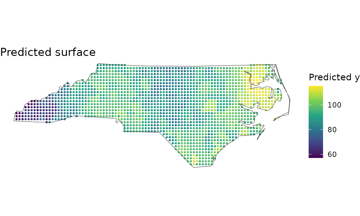

The fitted random forest predicted onto a regular grid over North Carolina and clipped to the state boundary, with predictions lowest in the far west and highest along the eastern coast.

A fitted model returns a number for any location you hand it, including locations whose predictor values look nothing like the training data. area_of_applicability() marks where the cross-validated score actually applies. Pass the folds you validated with:

aoa <- area_of_applicability(surf, model = rf_fit, folds = folds_blocked)

cat(sprintf("inside: %d | outside: %d | undetermined: %d | DI threshold %.3f\n",
            aoa$n_inside, aoa$n_outside, aoa$n_na, aoa$threshold))

## inside: 1645 | outside: 0 | undetermined: 0 | DI threshold 0.184

# AOA is NA wherever a predictor was missing or non-finite, and `!NA` is NA,
# which R silently skips in a subscripted assignment. Test for TRUE and let
# anything else count as outside.
inside <- aoa$aoa$AOA %in% TRUE
surf$.pred_masked <- ifelse(inside, surf$.pred, NA_real_)

ggplot() +
  geom_sf(data = surf, aes(colour = .pred_masked), size = 0.6) +
  geom_sf(data = nc_boundary, fill = NA, colour = "grey20") +
  scale_colour_viridis_c(name = "Predicted y", na.value = "grey85") +
  theme_void() +
  ggtitle("Predicted surface, extrapolations blanked out")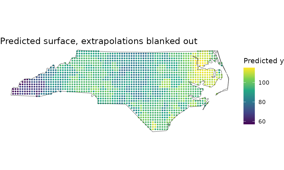

The same predicted surface with cells outside the area of applicability blanked out. Nothing is blanked, because the grid took its covariates from the nearest observation and so holds no combination the model had not already seen.

Nothing is masked here, and the reason is worth understanding rather than taking as reassurance: predict_surface(covariates = points_sf) copies predictor values from the nearest observation, so every grid cell carries a predictor vector some training point already had. Its dissimilarity index is therefore near zero by construction. The index earns its keep when the covariates come from somewhere else — a raster, a different survey, a future scenario. Hand it values outside the training range and it says so:

extreme <- st_sf(
  elevation   = c(mean(points_sf$elevation), max(points_sf$elevation) * 4),
  pop_density = c(mean(points_sf$pop_density), max(points_sf$pop_density) * 4),
  geometry    = st_geometry(points_sf)[1:2]
)
area_of_applicability(extreme, model = rf_fit, folds = folds_blocked)$aoa[, c("DI", "AOA")]

## Simple feature collection with 2 features and 2 fields
## Geometry type: POINT
## Dimension:     XY
## Bounding box:  xmin: 2604137 ymin: 653637.4 xmax: 2827401 ymax: 964007.8
## Projected CRS: NAD83 / North Carolina (ftUS)
##            DI   AOA                 geometry
## 1  0.04321651  TRUE POINT (2827401 653637.4)
## 2 15.00736636 FALSE POINT (2604137 964007.8)

Summary

Tessellation	Cells	Notes
Voronoi	40	Adapts to point density via k-means seeds
Hex grid	49	Uniform hexagons, good for regular sampling
Square grid	45	Simplest regular grid
Delaunay	586	One triangle per Delaunay triplet; finest resolution

The choropleths show how each tessellation aggregates the response. Section 5 shows the thing that matters most: on the same data and the same fitted model, the fold scheme moves the reported score substantially, and only the blocked number describes the task you actually have.

Where to go next

This page is the wide view. Each step has a vignette that stops and argues about it:

for	read
getting your own data in, and what the coordinates are in	`vignette("getting-started")`
how many cells, and the four criteria that disagree	`vignette("resolution")`
the five fold schemes, and sizing a block by measurement	`vignette("spatial-cross-validation")`
residual autocorrelation, aggregation standard errors, and two ways to leak	`vignette("diagnostics")`
handing the regions to someone else, and what to report	`vignette("reporting")`

Ten numbered scripts in system.file("scripts", package = "spatialkit") run the same ground at the console, printing what to look for in each figure before drawing it.

## R version 4.6.1 (2026-06-24)
## Platform: x86_64-pc-linux-gnu
## Running under: Ubuntu 24.04.5 LTS
## 
## Matrix products: default
## BLAS:   /usr/lib/x86_64-linux-gnu/openblas-pthread/libblas.so.3 
## LAPACK: /usr/lib/x86_64-linux-gnu/openblas-pthread/libopenblasp-r0.3.26.so;  LAPACK version 3.12.0
## 
## locale:
##  [1] LC_CTYPE=C.UTF-8       LC_NUMERIC=C           LC_TIME=C.UTF-8       
##  [4] LC_COLLATE=C.UTF-8     LC_MONETARY=C.UTF-8    LC_MESSAGES=C.UTF-8   
##  [7] LC_PAPER=C.UTF-8       LC_NAME=C              LC_ADDRESS=C          
## [10] LC_TELEPHONE=C         LC_MEASUREMENT=C.UTF-8 LC_IDENTIFICATION=C   
## 
## time zone: UTC
## tzcode source: system (glibc)
## 
## attached base packages:
## [1] stats     graphics  grDevices utils     datasets  methods   base     
## 
## other attached packages:
## [1] patchwork_1.3.2       ggplot2_4.0.3         dplyr_1.2.1          
## [4] sf_1.1-3              spatialkit_2.0.0.9000
## 
## loaded via a namespace (and not attached):
##  [1] GWmodel_2.4-1         tidyselect_1.2.1      viridisLite_0.4.3    
##  [4] farver_2.1.2          S7_0.2.2              fastmap_1.2.0        
##  [7] TH.data_1.1-5         digest_0.6.39         lifecycle_1.0.5      
## [10] LearnBayes_2.15.2     survival_3.8-6        magrittr_2.0.5       
## [13] compiler_4.6.1        rlang_1.3.0           sass_0.4.10          
## [16] tools_4.6.1           yaml_2.3.12           geometry_0.5.2       
## [19] data.table_1.18.6.1   knitr_1.52            FNN_1.1.4.1          
## [22] labeling_0.4.3        htmlwidgets_1.6.4     sp_2.2-3             
## [25] classInt_0.4-11       RColorBrewer_1.1-3    abind_1.4-8          
## [28] multcomp_1.4-32       KernSmooth_2.23-26    withr_3.0.3          
## [31] desc_1.4.3            grid_4.6.1            xts_0.14.3           
## [34] e1071_1.7-17          scales_1.4.0          MASS_7.3-65          
## [37] cli_3.6.6             mvtnorm_1.4-2         rmarkdown_2.32       
## [40] intervals_0.15.5      ragg_1.5.2            generics_0.1.4       
## [43] otel_0.2.0            robustbase_0.99-7     magic_1.6-1-1        
## [46] spdep_1.4-2           DBI_1.3.0             cachem_1.1.0         
## [49] proxy_0.4-29          splines_4.6.1         spatialreg_1.4-3     
## [52] parallel_4.6.1        s2_1.1.13             marginaleffects_1.0.0
## [55] vctrs_0.7.3           boot_1.3-32           Matrix_1.7-5         
## [58] sandwich_3.1-3        jsonlite_2.0.0        spData_2.3.5         
## [61] systemfonts_1.3.2     jquerylib_0.1.4       units_1.0-1          
## [64] glue_1.8.1            pkgdown_2.2.1         DEoptimR_1.2-2       
## [67] codetools_0.2-20      gstat_2.1-6           gtable_0.3.6         
## [70] deldir_2.0-4          tibble_3.3.1          logger_0.4.3         
## [73] pillar_1.11.1         htmltools_0.5.9       R6_2.6.1             
## [76] wk_0.9.5              textshaping_1.0.5     evaluate_1.0.5       
## [79] lattice_0.22-9        backports_1.5.1       bslib_0.12.0         
## [82] class_7.3-23          Rcpp_1.1.2            coda_0.19-4.1        
## [85] nlme_3.1-169          spacetime_1.3-4       ranger_0.18.0        
## [88] xfun_0.61             fs_2.1.0              zoo_1.9-1            
## [91] pkgconfig_2.0.3

Justin Chase

30 September 2026

Overview

1. Packages and boundary

2. Synthetic observations

3. Four tessellations

3a. Voronoi from ~40 k-means seeds

3b and 3c. Hex and square grids (~50 cells)

3d. Delaunay triangles

4. Cell-level aggregation with `summarize_by_cell()`

Choropleths

5. Spatial cross-validation

5a. How far does correlation reach?

5b. Two fold schemes on the same data

5c. The number the fold scheme changes

6. Fitting a model

Residual diagnostics

GWR, if `GWmodel` is installed

Comparing backends on identical folds

7. From a fit to a map, and where the map applies

Summary

Where to go next

spatialkit: Tessellations, Spatial Cross-Validation and Models

Justin Chase

30 September 2026

Overview

1. Packages and boundary

2. Synthetic observations

3. Four tessellations

3a. Voronoi from ~40 k-means seeds

3b and 3c. Hex and square grids (~50 cells)

3d. Delaunay triangles

4. Cell-level aggregation with summarize_by_cell()

Choropleths

5. Spatial cross-validation

5a. How far does correlation reach?

5b. Two fold schemes on the same data

5c. The number the fold scheme changes

6. Fitting a model

Residual diagnostics

GWR, if GWmodel is installed

Comparing backends on identical folds

7. From a fit to a map, and where the map applies

Summary

Where to go next

4. Cell-level aggregation with `summarize_by_cell()`

GWR, if `GWmodel` is installed