Diagnostics

Justin Chase

30 September 2026

This article needs two optional packages: gstat, which fits the variogram behind the autocorrelation range, and ggplot2 for the figures. When either is missing the code is shown but not run, and a note at the top says so.

Four questions a score does not answer

A cross-validated RMSE tells you how far the predictions fell from the held-out values. It is silent on four things that decide whether the analysis holds up: whether the model left spatial structure in its residuals, whether the standard errors on aggregated values are the width they claim, whether a cell mean is the best estimate of that cell available, and where on the map the score applies at all. A fifth section shows two ways the score itself can be wrong.

A fixture and a model that is wrong in a known way

The response is driven by one real predictor and by a spatial field the model never sees. b is noise. A linear model on a and b therefore leaves the field in its residuals, which is what the first diagnostic should detect.

library(sf)
library(spatialkit)

set.seed(11)
n  <- 350
xy <- data.frame(x = 5e5 + runif(n, 0, 1000), y = 5e6 + runif(n, 0, 1000))
D  <- as.matrix(dist(xy))
field <- as.numeric(t(chol(exp(-D / 70) + diag(1e-8, n))) %*% rnorm(n))
xy$a  <- rnorm(n)
xy$b  <- rnorm(n)
xy$z  <- 1.5 * xy$a + field + rnorm(n, sd = 0.3)
pts   <- st_as_sf(xy, coords = c("x", "y"), crs = 32632)

lm_fit <- function(train_sf, response_var = "z", predictor_vars = c("a", "b")) {
  d   <- st_drop_geometry(train_sf)
  # With no predictors the model is intercept-only: "z ~ 1", not "z ~ ".
  rhs <- if (length(predictor_vars)) paste(predictor_vars, collapse = " + ") else "1"
  fml <- as.formula(paste(response_var, "~", rhs))
  new_spatial_fit(
    subclass       = "lmsurf_fit",
    engine         = lm(fml, data = d),
    formula        = fml,
    response_var   = response_var,
    predictor_vars = predictor_vars,
    data_sf        = train_sf
  )
}
predict.lmsurf_fit <- function(object, newdata = NULL, ...) {
  if (is.null(newdata)) return(fitted(object$engine))
  as.numeric(predict(object$engine, newdata = st_drop_geometry(newdata)))
}
residuals.lmsurf_fit <- function(object, ...) residuals(object$engine)
fitted.lmsurf_fit    <- function(object, ...) fitted(object$engine)
for (g in c("predict", "residuals", "fitted"))
  registerS3method(g, "lmsurf_fit", get(paste0(g, ".lmsurf_fit")))

fit <- lm_fit(pts)

1. Structure left in the residuals

mi <- residual_morans_i(fit)
mi

## Residual Moran's I = 0.4480   (E[I] = -0.0029, sd = 0.0253)
##   z = 17.841, p = 3.38e-71
##   null: residual moments, exact for these residuals; n = 350, df = 347, design rank 3
##   residual kurtosis 3.152 (3 = Gaussian)
##   weights: 350 x 350 dgCMatrix, 8 neighbour(s) per row; not retained, keep_weights = TRUE to keep it

A large positive Moran’s I says nearby residuals resemble each other, so the model is missing something that varies smoothly across the map. Here that is the simulated field, by construction.

Three parts of the print earn attention. The null says which moments the p-value came from: residual moments condition on the design matrix and are exact for OLS residuals, randomisation moments treat the residuals as exchangeable and are an approximation for any model. null = "auto" chooses per fit, so read what it chose. The design rank is the rank of the rebuilt model matrix, which is where the residual degrees of freedom come from. The kurtosis says how far the residuals sit from the Gaussian case the moments assume, with 3 as the reference.

The weight matrix is $n \times n$ and is described instead of returned. Ask for it when you want to reuse the same neighbours:

mi_w <- residual_morans_i(fit, keep_weights = TRUE)
dim(mi_w$weights)

## [1] 350 350

mi$weights_summary[c("n", "storage", "neighbours", "kept")]

## $n
## [1] 350
## 
## $storage
## [1] "dgCMatrix"
## 
## $neighbours
## [1] 8 8
## 
## $kept
## [1] FALSE

weights_summary is present either way, so a NULL in weights is always explained.

2. Standard errors on aggregated values

Aggregate the points into cells and the naive standard error of each cell mean is $s/\sqrt{n}$, which treats the points in a cell as independent. For the cell’s own mean that is the right standard error when the points are spread through the cell. For the cell mean as an estimate of the population (grand) mean it is not: on an autocorrelated field the points in a cell share the cell’s departure from that mean, and the effective sample size is smaller than the count.

hull <- clip_target_for(pts, expand = 0.02, quiet = TRUE)
tess <- build_tessellation(pts, boundary = hull, method = "square",
                           approx_n_cells = 24, quiet = TRUE)
asg  <- assign_features_to_polygons(pts, tess$cells)

c(cells = nrow(tess$cells), points = nrow(asg),
  median_per_cell = median(table(asg$poly_id)))

##           cells          points median_per_cell 
##              25             350              14

summarize_by_cell() takes a design effect, and three settings are worth comparing on the same cells.

sac  <- estimate_sac_range(pts, "z")
iid  <- summarize_by_cell(asg, "z", cells_sf = tess$cells, deff = 1)
kish <- summarize_by_cell(asg, "z", cells_sf = tess$cells, deff = "kish")
vgm  <- summarize_by_cell(asg, "z", cells_sf = tess$cells, deff = "variogram",
                          sac = sac)

data.frame(n         = iid$n,
           iid       = round(iid$..se_resp_z, 3),
           kish      = round(kish$..se_resp_z, 3),
           variogram = round(vgm$..se_resp_z, 3))[1:5, ]

##    n   iid  kish variogram
## 1 14 0.546 1.072     1.272
## 2 11 0.447 0.805     0.963
## 3 18 0.381 0.822     0.987
## 4 16 0.592 1.222     1.467
## 5  8 0.527 0.854     0.996

The median cell’s standard error is 1.96 times wider under kish and 2.35 times wider under variogram than the independent-sampling one. As an estimate of the population mean, a confidence interval built on the naive number is about half the width it should be on this field. For the cell’s own mean the naive standard error is the right one, and section 3 (kriging_adequacy()) covers that quantity.

deff = "kish" estimates an intra-class correlation from the within-cell and between-cell variance and applies Kish’s factor. deff = "variogram" takes the correlation from the fitted variogram model, so it uses the spatial structure rather than the cell labels. The choice is recorded:

str(attr(vgm, "deff_applied"))

## List of 6
##  $ method   : chr "variogram"
##  $ deff     : num [1:25] 4.12 3.49 5.11 4.65 2.71 ...
##  $ deff_rows: num [1:25] 4.12 3.49 5.11 4.65 2.71 ...
##  $ rbar     : num [1:25] 0.24 0.249 0.242 0.243 0.244 ...
##  $ crs      :List of 2
##   ..$ input: chr "EPSG:32632"
##   ..$ wkt  : chr "PROJCRS[\"WGS 84 / UTM zone 32N\",\n    BASEGEOGCRS[\"WGS 84\",\n        ENSEMBLE[\"World Geodetic System 1984 "| __truncated__
##   ..- attr(*, "class")= chr "crs"
##  $ max_n    : int 500

attr(kish, "icc")$resp

## [1] 0.1692353

A cell whose design effect reaches its point count carries no information about the variance at all, and its standard error is NA. That is a statement about the cell, so the fix is bigger cells or more points, not a different setting.

3. Is the cell mean the best estimate of the cell?

The plain mean weights every point in a cell equally and ignores everything outside it. Block kriging uses the fitted variogram, borrows from neighbouring cells, and reports a variance derived from the spatial model. kriging_adequacy() runs both and compares them.

ka <- kriging_adequacy(asg, "z", tess$cells, k = 4, seed = 1)
ka

## Block-kriging adequacy over 25 cells (350 points, nmax 50)
##   variogram: Nug(2.34, 0) + Exp(1.49, 208); sill 3.83, nugget 2.34 (61%), range 623.7
##   kriging variance / no-data variance of the cell mean (1 = nothing from the data): median 0.130, range 0.090-0.217; 0 cell(s) above 0.5
##   kriging variance exceeds s^2/n in 4 of the 25 cell(s) with two or more points
##   kriged minus plain mean: |shift| > 1 SE in 4 of 25 cell(s), > 2 SE in 0
##   empty cells: 0 (kriged estimate and variance available for each)
##   blocked CV (block_kfold, 4 folds, 350 points): var of standardised error 0.96 (1 = kriging variance correct; above 1 = understated), mean -0.04, RMSE 1.76

Three readings. kr_var against the naive se^2 says whether the naive standard error was optimistic. kr_shift is how far the kriged estimate moved from the plain mean, in units of the naive standard error, and a shift beyond one or two of those says the mean and the spatial model disagree about that cell. The blocked cross-validation at the end standardises each held-out error by its kriging variance: a variance of 1 means the kriging variance is right, and above 1 means it is understated.

head(st_drop_geometry(ka)[, c("n", "mean", "se", "kr_pred", "kr_var", "kr_shift")], 4)

## Block-kriging adequacy (subset; the fitted summary is not carried by a subset)
##    n      mean        se   kr_pred    kr_var   kr_shift
## 1 14 1.1020196 0.5463243 0.9482019 0.1388294 -0.2815501
## 2 11 0.3804887 0.4470487 0.5214361 0.1528287  0.3152841
## 3 18 1.0791003 0.3805235 0.8801156 0.1183915 -0.5229235
## 4 16 1.5055114 0.5920044 1.2414298 0.1078660 -0.4460805

An empty cell still gets a kriged estimate and variance, which is the practical reason to run this: a tessellation fine enough to be useful usually has cells with no observation in them. This grid has none, as the report’s empty cells line says, because 25 cells over 350 points leaves every cell populated; the reporting vignette’s grid over the North Carolina counties has six.

4. Where the score applies

A cross-validated number describes the region the training data covers. For predictions made anywhere else, it describes nothing. area_of_applicability() marks the difference, following Meyer and Pebesma (2021).

grid <- create_grid_polygons(hull, target_cells = 200, type = "square")
gp   <- suppressWarnings(st_centroid(grid))
set.seed(2)
gp$a <- rnorm(nrow(gp))
gp$b <- rnorm(nrow(gp), mean = 3)     # shifted well outside the training range

aoa <- area_of_applicability(gp, model = fit)
aoa

## Area of applicability (Meyer & Pebesma 2021)
## 
##   predictors  : 2 (a, b)
##   weighted    : no (all predictors count equally)
##   training    : 350 points
##   reference   : nearest other training point (no folds supplied)
##   normaliser  : 1.7610 (mean pairwise distance)
##   threshold   : 0.1552 (outlier-removed max of training DI)
## 
##   64 of 225 prediction points inside the AOA (28.4%)
## 
## Predictions outside the AOA are extrapolations; the cross-validated
## performance estimate does not cover them.

plot(aoa)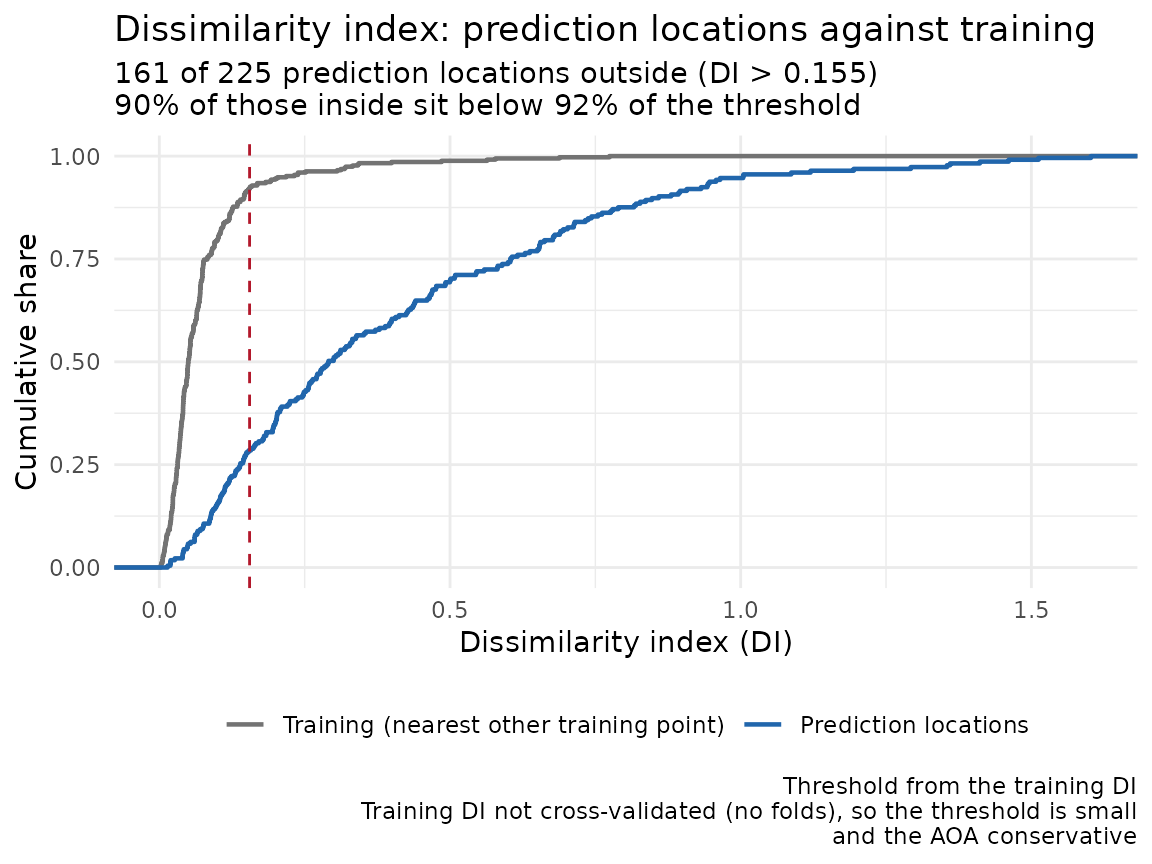

Shifting one predictor three standard deviations moves most of the grid outside the domain the model was trained on. The dissimilarity index DI is on aoa$aoa, alongside the logical AOA, and threshold is the cutoff derived from the training data.

One trap worth stating plainly. AOA is NA wherever a predictor was missing or non-finite, !NA is NA, and R skips NA positions in a subscripted assignment. Test for TRUE:

inside <- !is.na(aoa$aoa$AOA) & aoa$aoa$AOA
c(inside = sum(inside), outside_or_unknown = sum(!inside))

##             inside outside_or_unknown 
##                 64                161

5. Two ways to leak

Coordinates as predictors. A model given x and y can reproduce the training surface by memorising location, and random folds will not detect it. fit_rf_model(include_coords = TRUE) logs a caution (once per session) for this reason. Score any such model with blocked folds, and read vignette("spatial-cross-validation") for what the blocking has to be wide enough to do.

Selection outside the fold. Choosing predictors on the whole data set and then cross-validating the chosen set gives the selection a look at every test row. select_features_forward() does the selection inside the resampling, and it takes the fold scheme as an argument for the same reason the outer loop does. Blocked folds only keep test rows apart from training rows if the blocks are at least as wide as the autocorrelation range. make_folds() estimates that range for what the candidates leave unexplained, about 330 m on this field, and warns when the blocks are narrower. The default grid here has blocks about 250 m across, so block_size = 400 is passed:

# select_features_forward() calls fit_fn(train_sf, vars), so the learner above
# needs an adapter that puts `vars` in the predictor slot. Step 0 fits it with
# no predictors at all, which is why lm_fit() builds "z ~ 1" for an empty set.
sel_fn <- function(train_sf, vars) lm_fit(train_sf, "z", vars)

sel <- select_features_forward(pts, "z", c("a", "b"), fit_fn = sel_fn,
                               k = 4, method = "block_kfold",
                               block_size = 400, seed = 1)
sel$selected

## [1] "a"

sel$history

##   step variable    score n_pred
## 1    0   <none> 1.886912    350
## 2    1        a 1.113470    350
## 3    1        b 1.887999    350
## 4    2        b 1.116468    350

history has one row per candidate scored at each step. Step 0 is the intercept-only model, so a had to beat it to be added, and at step 2 adding the noise variable b made the cross-validated RMSE slightly worse, so the selection stopped at a. With tol set, a candidate has to improve the score by more than tol, from step 1 on.

Its inner folds default to the scheme you pass. Passing random_kfold there logs a caution, because a leaky inner loop can select a variable for being spatially close to the response and an honest outer loop will then report a respectable number for a dishonestly chosen feature set.

Next

vignette("spatial-cross-validation") covers fold schemes and block sizing. vignette("resolution") covers choosing the cell count these diagnostics are computed over. ?residual_morans_i documents the two nulls and when each is exact, ?summarize_by_cell derives the design-effect correction and reports its measured coverage, and ?area_of_applicability covers the weighting and the threshold.