What to save, and what to report

The other vignettes each take one decision: how many cells, which fold scheme, which diagnostic. This one starts after those are settled. You have regions and a validated model, and two things have to leave your session: the regions, in a form someone else can open and join to, and the numbers that say how far the map they are looking at can be trusted.

Everything here runs on the hard dependencies, with two exceptions that skip themselves with a note when absent: ggplot2 draws the one map, and gstat fits the variogram in the second half.

The regions as a file someone else can use

North Carolina’s counties, with the 1974 SIDS rate per thousand births, and a hexagonal grid of regions drawn from where the counties are rather than from the county boundaries themselves. Twelve cells are asked for; a grid clipped to an irregular outline returns more, and the count that comes back is the one to quote.

library(sf)
library(spatialkit)

nc <- st_read(system.file("shape/nc.shp", package = "sf"), quiet = TRUE)
counties <- ensure_projected(nc[, c("NAME", "BIR74", "SID74")])
counties$rate <- 1000 * counties$SID74 / counties$BIR74

centres  <- coerce_to_points(counties)
boundary <- clip_target_for(centres, expand = 0.01)
regions  <- build_tessellation(centres, method = "hex", approx_n_cells = 12,
                               boundary = boundary)$cells
nrow(regions)

## [1] 18

approx_n_cells is approximate, as its name says: hexagons over this bounding box came out at 18 for a request of 12, and some of them will hold no counties at all.

Grouping a layer you already have

assign_features_to_polygons() is usually shown on points, but it takes polygons too. largest = TRUE gives each county to the region it overlaps most, which is what makes the result a grouping: one row per county, never a county split across two rows.

grouped <- assign_features_to_polygons(counties, regions,
                                       polygon_id_col = "cell_id",
                                       largest = TRUE)

c(counties_in = nrow(counties), rows_out = nrow(grouped),
  regions_used = length(unique(stats::na.omit(grouped$cell_id))))

##  counties_in     rows_out regions_used 
##          100          100           12

range(table(grouped$cell_id))

## [1]  2 13

100 counties in, 100 rows out, spread over 12 of the 18 regions, from 2 to 13 counties each. That row-count equality is the property to check after any grouping: sf::st_join() would have duplicated every county that touches two regions, and the counts per region would then be wrong by however many counties straddle a border.

summarize_by_cell() reduces the grouped layer to one row per region, and passing cells_sf keeps the geometry and the empty regions:

cells <- summarize_by_cell(grouped, response_var = "rate", id_col = "cell_id",
                           cells_sf = regions, conf_level = 0.95)

names(cells)

##  [1] "cell_id"           "n"                 "resp_mean_rate"   
##  [4] "..sd_resp_rate"    "..se_resp_rate"    "..neff_resp_rate" 
##  [7] "..df_resp_rate"    "..ci_lo_resp_rate" "..ci_hi_resp_rate"
## [10] "cell_weight"       "geometry"

sum(is.na(cells$n))

## [1] 6

6 of the 18 regions are empty, carrying NA rather than being silently dropped. A region with no data in it is a fact about the map, and one worth keeping: it is where the model has nothing to stand on.

library(ggplot2)

ggplot() +
  geom_sf(data = cells, aes(fill = resp_mean_rate), colour = "white") +
  geom_sf(data = counties, fill = NA, colour = "grey70", linewidth = 0.2) +
  scale_fill_viridis_c(name = "SIDS rate\nper 1,000", na.value = "grey92") +
  labs(title = "Counties grouped into data-drawn regions",
       subtitle = sprintf("%d regions, %d populated; grey = no county inside",
                          nrow(cells), sum(!is.na(cells$n)))) +
  theme_void()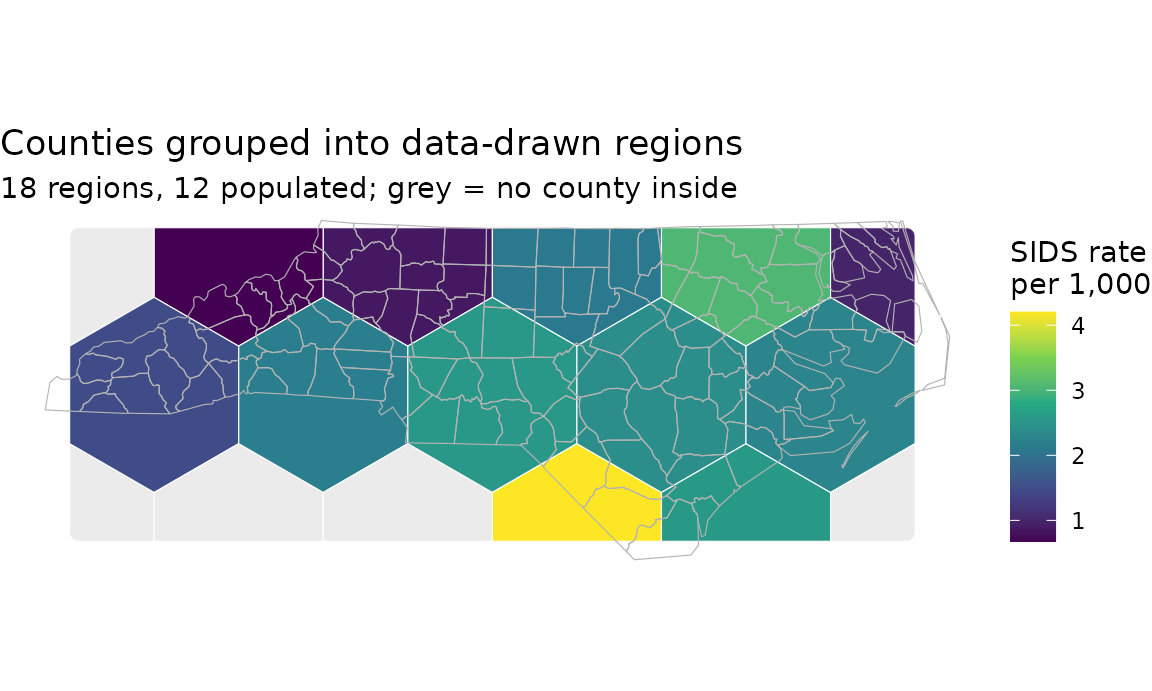

The North Carolina counties grouped into eighteen hexagonal regions, each shaded by the mean 1974 SIDS rate of the counties inside it. County outlines show underneath. Six regions along the edges hold no county and are grey.

Is this location inside?

The question the regions get asked most often once they leave your session is whether some new location falls in one. That is the same function with keep_unassigned = TRUE, which returns one row per location and NA for anything outside every region.

sites <- st_as_sf(
  data.frame(site = c("Raleigh", "Wilmington", "Atlantic", "Norfolk VA"),
             lon  = c(-78.64, -77.95, -74.50, -76.29),
             lat  = c( 35.78,  34.23,  35.00,  36.85)),
  coords = c("lon", "lat"), crs = 4326)

inside <- assign_features_to_polygons(st_transform(sites, st_crs(regions)),
                                      regions, polygon_id_col = "cell_id",
                                      keep_unassigned = TRUE)
st_drop_geometry(inside)

##         site cell_id
## 1    Raleigh      13
## 2 Wilmington      14
## 3   Atlantic      NA
## 4 Norfolk VA      NA

2 of the 4 sit inside a region. The default is keep_unassigned = FALSE, which drops them instead; that is the right default when you are aggregating, and the wrong one when you are answering a membership question, because a dropped row looks like a location you never asked about.

Two details decide whether the answer is meaningful. The locations have to be in the regions’ CRS, which is why st_transform() is there: the regions are in whatever projection ensure_projected() chose, and lon/lat degrees compared against metres will put everything outside. And a point on a shared border falls in both cells, so tie_break decides which one it is recorded in; see ?assign_features_to_polygons for the rules.

IDs that survive a reprojection

The cell_id a tessellation carries is already derived from the geometry, so it does not change when the input points arrive in another order. What it is not is portable: a file that has been reprojected, re-sorted and re-read elsewhere has no memory of how it was built. ensure_stable_poly_id() derives an ID from the geometry itself, in a common CRS, so the same region gets the same ID from whoever computes it, in whatever projection the file is in by then. The exception is fine cells stacked within about a centimetre of the same longitude, which a reprojection can swap (see ?ensure_stable_poly_id); regions this size are nowhere near it.

regions$src <- seq_len(nrow(regions))

from_projected <- ensure_stable_poly_id(regions[, "src"])
from_lonlat    <- ensure_stable_poly_id(st_transform(regions[, "src"], 4326))

identical(from_projected$poly_id[order(from_projected$src)],
          from_lonlat$poly_id[order(from_lonlat$src)])

## [1] TRUE

Use that column, not the row position, as the key anything downstream joins on.

Writing it out

The regions are an ordinary sf layer, so sf::st_write() handles them. The format matters more than it looks:

dir <- tempfile(); dir.create(dir)

st_write(cells, file.path(dir, "regions.gpkg"), quiet = TRUE)
gpkg <- st_read(file.path(dir, "regions.gpkg"), quiet = TRUE)

suppressWarnings(st_write(cells, file.path(dir, "regions.shp"), quiet = TRUE))
shp <- st_read(file.path(dir, "regions.shp"), quiet = TRUE)

attr_names <- function(x) setdiff(names(x), attr(x, "sf_column"))
kept <- function(x) length(intersect(attr_names(x), attr_names(cells)))

c(columns = length(attr_names(cells)),
  GeoPackage = kept(gpkg), Shapefile = kept(shp))

##    columns GeoPackage  Shapefile 
##         10         10          2

##  [1] "cell_id"  "n"        "rsp_mn_"  "X__sd_r_" "X__s_rs_" "X__nff__"
##  [7] "X__df_r_" "X__c_l__" "X__c_h__" "cll_wgh"

A shapefile field name is capped at ten characters, so the standard errors and confidence bounds arrive as X__s_rs_ and X__c_l__: of the 10 columns summarize_by_cell() produced, 2 survive the trip. GeoPackage keeps every one of them, and renames only the geometry column, which is a GeoPackage convention. Write a GeoPackage unless something downstream can only read shapefiles, and if it can only read shapefiles, rename the columns yourself first so you choose the abbreviations.

The numbers the run already recorded

Nothing below is recomputed for the report. Each of these is written into the object at the time the decision was made, which is the point: a report assembled from $params and $info describes the run that happened rather than a reconstruction of it.

The counties carry a real response, but a weak one, so the rest of this vignette runs on a simulated field over the same county centres, with a known correlation length of 120 km:

set.seed(42)
xy    <- st_coordinates(centres)
D     <- as.matrix(dist(xy))
field <- as.numeric(t(chol(exp(-D / 120e3) + diag(1e-8, nrow(D)))) %*%
                      rnorm(nrow(D)))

pts <- centres
pts$elev <- rnorm(nrow(pts))
pts$z    <- 0.8 * pts$elev + 2 * field + rnorm(nrow(pts), sd = 0.3)

# A learner with no optional dependencies: a linear trend surface in the
# coordinates, plus the one covariate.
trend_fit <- function(train_sf, ...) {
  d  <- st_drop_geometry(train_sf)
  co <- st_coordinates(train_sf)
  d$x <- co[, 1]; d$y <- co[, 2]
  new_spatial_fit(subclass = "trend_fit",
                  engine = stats::lm(z ~ elev + x + y, data = d),
                  formula = z ~ elev + x + y, response_var = "z",
                  predictor_vars = "elev", data_sf = train_sf)
}
predict.trend_fit <- function(object, newdata = NULL, ...) {
  if (is.null(newdata)) return(stats::fitted(object$engine))
  d  <- st_drop_geometry(newdata)
  co <- st_coordinates(newdata)
  d$x <- co[, 1]; d$y <- co[, 2]
  as.numeric(stats::predict(object$engine, newdata = d))
}
residuals.trend_fit <- function(object, ...) stats::residuals(object$engine)
fitted.trend_fit    <- function(object, ...) stats::fitted(object$engine)
for (.g in c("predict", "residuals", "fitted"))
  registerS3method(.g, "trend_fit", get(paste0(.g, ".trend_fit")))

folds <- make_folds(pts, k = 5, method = "block_kfold", block_size = 100e3,
                    seed = 1)
cv    <- cv_spatial(pts, "z", "elev", trend_fit, folds = folds)
fit   <- trend_fit(pts)

A worked report

Six items. Every one is read out of an object the run already produced.

m <- function(x) format(round(as.numeric(x)), big.mark = ",", scientific = FALSE)

report <- list(
  folds = sprintf("%s, k = %d, %d x %d blocks of %s m (%s)",
                  folds$method, folds$k, folds$params$grid_nx,
                  folds$params$grid_ny, m(folds$params$block_size),
                  folds$params$crs),
  score = sprintf("RMSE %.2f (per fold %.2f to %.2f), R2 %.3f",
                  cv$overall$RMSE, min(cv$fold_metrics$RMSE),
                  max(cv$fold_metrics$RMSE), cv$overall$R2),
  coverage = sprintf("%d of %d folds scored, %d rows dropped, %d orphan, %d unknown id",
                     cv$n_folds_succeeded, cv$n_folds_attempted, cv$n_dropped,
                     length(cv$orphan_rows), cv$n_unknown_ids)
)

mi <- residual_morans_i(fit)
report$residuals <- sprintf("Moran's I %.3f (z = %.1f, p = %.3g, %s null)",
                            mi$observed, mi$z, mi$p_value, mi$null)

surface <- predict_surface(fit, n_cells = 1500, covariates = pts,
                           boundary = counties)
aoa <- area_of_applicability(surface, model = fit, folds = folds)
report$applicability <- sprintf("%d of %d prediction cells outside (DI > %.3f)",
                                aoa$n_outside, aoa$n_new, aoa$threshold)

sac <- estimate_sac_range(pts, "z")
report$range <- sprintf("estimated range %s m against blocks of %s m",
                        m(sac), m(folds$params$block_size))

cat(paste0("- ", names(report), ": ", unlist(report)), sep = "\n")

## - folds: block_kfold, k = 5, 7 x 2 blocks of 100,000 m (+proj=aea +lat_1=34.333391 +lat_2=36.138461 +lat_0=35.559467 +lon_0=-79.400417 +datum=WGS84 +units=m +no_defs)
## - score: RMSE 2.25 (per fold 1.97 to 2.61), R2 -0.063
## - coverage: 5 of 5 folds scored, 0 rows dropped, 0 orphan, 0 unknown id
## - residuals: Moran's I 0.567 (z = 12.6, p = 3.62e-36, randomisation null)
## - applicability: 0 of 937 prediction cells outside (DI > 0.073)
## - range: estimated range 286,804 m against blocks of 100,000 m

Read together, those lines say the run failed its own checks, which is what a report is for.

The blocks are 100,000 m across and the correlation reaches about 286,804 m, so training and test data sit inside one correlation length of each other. The score is still optimistic, and the fix is blocks at least as wide as the range, or auto_range = TRUE to size them from it.

The cross-validated R2 of -0.063 is below zero, which says the trend surface predicts held-out blocks worse than their own mean does, and Moran’s I of 0.57 on the residuals (z = 12.6) says why: most of the structure in z is the field, and a plane in the coordinates cannot represent it. That is the point at which you fit something spatial rather than report this.

The applicability line reads 0 of 937 here because predict_surface() joined the covariate from the nearest observation, so no grid cell holds a combination the model never saw. On a real covariate raster it will not be zero; vignette("diagnostics") works through what to do when it is not.

What each line is for

Report	From	Because
The fold scheme, the block size and the estimated range, in named CRS units	`folds$params`	A cross-validation score means nothing without the geometry that produced it: blocks below the range leak, and the score comes back flattering (Roberts et al. 2017)
The metric with its per-fold spread, not the pooled value alone	`cv$fold_metrics`, `plot_cv_metrics()`	0.9 in four folds and 14 in one is a model that fails in one region, and the pooled number cannot tell that from uniform mediocrity
Residual Moran’s I with its null	`residual_morans_i()`	It is the check on whether the spatial structure the model was built for actually got modelled
The share of the prediction area outside the area of applicability	`area_of_applicability()`	A fitted model returns a number everywhere, including ground nothing like its training data, and the CV score does not apply there (Meyer and Pebesma 2021)
Interval coverage, for a model with intervals	`cv_bayes()`, `plot_calibration()`	Good point predictions routinely come with badly calibrated intervals, so RMSE alone can prefer the model whose uncertainty is wrong (Heaton et al. 2019)
Rows dropped, folds that failed, orphan and unknown IDs	`cv$n_dropped`, `cv$orphan_rows`, `cv$fold_status`	A score computed over 80 percent of the data is not a score over the data, and nothing else in the output says so

Two of the six are about what the number does not cover, which is the part that gets left out. The area of applicability bounds the map in space and the dropped-row counts bound it in sample: without them a reader has a figure and no idea what it was computed over.

For the aggregates themselves, report the standard error that comes with each cell mean rather than the mean alone. summarize_by_cell() computes it with the observation count beside it. For per-region values like the map above, that is the default deff = 1 standard error used here (or the block-kriging variance, kr_var, from kriging_adequacy()). A deff setting widens it for within-cell autocorrelation, which is right only when the regional means feed a claim about the population (here statewide) mean; ?summarize_by_cell says which is which. A cell mean from two observations and one from thirteen are different claims, and printed side by side they look identical.

populated <- cells[!is.na(cells$n), ]
summary(populated$n)

##    Min. 1st Qu.  Median    Mean 3rd Qu.    Max. 
##   2.000   5.750   9.500   8.333  11.000  13.000

range(populated$..se_resp_rate, na.rm = TRUE)

## [1] 0.1616037 0.6601569

What to save

Enough to rerun it, which is less than it sounds:

the seed (folds$params$seed) and the fold assignment (folds$assignment),
the regions, with ensure_stable_poly_id() applied, as a GeoPackage,
folds$params and the fit’s $info, which hold every decision made for you,
the session’s package versions.

The regions are the one output that cannot be regenerated from the others without care. get_voronoi_seeds() and the k-means sweep in determine_optimal_levels() are seeded, so they repeat, but only at the same seed and the same package version. Save the layer.

vignette("getting-started") is the shortest path through the pipeline that produced all of this. vignette("diagnostics") covers the residual and applicability checks the table asks you to report, and vignette("spatial-cross-validation") covers fold geometry and how to read a CV result down to the last row.

References

Heaton, M. J., Datta, A., Finley, A. O., et al. (2019). A case study competition among methods for analyzing large spatial data. Journal of Agricultural, Biological and Environmental Statistics 24, 398-425. https://doi.org/10.1007/s13253-018-00348-w

Meyer, H. and Pebesma, E. (2021). Predicting into unknown space? Estimating the area of applicability of spatial prediction models. Methods in Ecology and Evolution 12(9), 1620-1633. https://doi.org/10.1111/2041-210X.13650

Roberts, D. R., Bahn, V., Ciuti, S., et al. (2017). Cross-validation strategies for data with temporal, spatial, hierarchical, or phylogenetic structure. Ecography 40(8), 913-929. https://doi.org/10.1111/ecog.02881

## R version 4.6.1 (2026-06-24)
## Platform: x86_64-pc-linux-gnu
## Running under: Ubuntu 24.04.5 LTS
## 
## Matrix products: default
## BLAS:   /usr/lib/x86_64-linux-gnu/openblas-pthread/libblas.so.3 
## LAPACK: /usr/lib/x86_64-linux-gnu/openblas-pthread/libopenblasp-r0.3.26.so;  LAPACK version 3.12.0
## 
## locale:
##  [1] LC_CTYPE=C.UTF-8       LC_NUMERIC=C           LC_TIME=C.UTF-8       
##  [4] LC_COLLATE=C.UTF-8     LC_MONETARY=C.UTF-8    LC_MESSAGES=C.UTF-8   
##  [7] LC_PAPER=C.UTF-8       LC_NAME=C              LC_ADDRESS=C          
## [10] LC_TELEPHONE=C         LC_MEASUREMENT=C.UTF-8 LC_IDENTIFICATION=C   
## 
## time zone: UTC
## tzcode source: system (glibc)
## 
## attached base packages:
## [1] stats     graphics  grDevices utils     datasets  methods   base     
## 
## other attached packages:
## [1] ggplot2_4.0.3         spatialkit_2.0.0.9000 sf_1.1-3             
## 
## loaded via a namespace (and not attached):
##  [1] s2_1.1.13          sass_0.4.10        generics_0.1.4     class_7.3-23      
##  [5] KernSmooth_2.23-26 lattice_0.22-9     digest_0.6.39      magrittr_2.0.5    
##  [9] evaluate_1.0.5     grid_4.6.1         RColorBrewer_1.1-3 fastmap_1.2.0     
## [13] Matrix_1.7-5       jsonlite_2.0.0     e1071_1.7-17       DBI_1.3.0         
## [17] viridisLite_0.4.3  scales_1.4.0       textshaping_1.0.5  jquerylib_0.1.4   
## [21] cli_3.6.6          rlang_1.3.0        units_1.0-1        intervals_0.15.5  
## [25] withr_3.0.3        cachem_1.1.0       yaml_2.3.12        otel_0.2.0        
## [29] FNN_1.1.4.1        tools_4.6.1        dplyr_1.2.1        spacetime_1.3-4   
## [33] logger_0.4.3       vctrs_0.7.3        R6_2.6.1           zoo_1.9-1         
## [37] proxy_0.4-29       lifecycle_1.0.5    classInt_0.4-11    fs_2.1.0          
## [41] htmlwidgets_1.6.4  ragg_1.5.2         pkgconfig_2.0.3    desc_1.4.3        
## [45] pkgdown_2.2.1      pillar_1.11.1      bslib_0.12.0       gtable_0.3.6      
## [49] Rcpp_1.1.2         glue_1.8.1         gstat_2.1-6        systemfonts_1.3.2 
## [53] xfun_0.61          tibble_3.3.1       tidyselect_1.2.1   knitr_1.52        
## [57] farver_2.1.2       htmltools_0.5.9    labeling_0.4.3     rmarkdown_2.32    
## [61] xts_0.14.3         wk_0.9.5           compiler_4.6.1     S7_0.2.2          
## [65] sp_2.2-3

Justin Chase

30 September 2026