Spatial cross-validation

Justin Chase

30 September 2026

This article needs two optional packages: gstat, which fits the variogram behind the autocorrelation range, and ggplot2 for the figures. When either is missing the code is shown but not run, and a note at the top says so.

The problem with a random fold

A random fold puts a test point’s neighbours in the training set. When the field is spatially autocorrelated, those neighbours carry the test point’s value, and a model with any capacity to memorise location will look up the answer. The cross-validation score then measures interpolation between nearby training points, and reports it as a prediction error for ground the model has never seen.

Everything else in this vignette follows from wanting a number that does not do that.

A learner you can read

The effect is easiest to see with a model whose memorising is obvious. new_spatial_fit() is the extension point for putting your own learner on the package’s folds, and five-nearest-neighbour smoothing is about the simplest thing that fits through it.

library(sf)
library(spatialkit)

knn_fit <- function(train_sf, response_var = "z", k = 5L) {
  new_spatial_fit(
    subclass       = "knnsurf_fit",
    engine         = list(xy = st_coordinates(train_sf),
                          y = st_drop_geometry(train_sf)[[response_var]],
                          k = k),
    formula        = as.formula(paste(response_var, "~ 1")),
    response_var   = response_var,
    predictor_vars = character(0),
    data_sf        = train_sf
  )
}

predict.knnsurf_fit <- function(object, newdata = NULL, ...) {
  e  <- object$engine
  xy <- if (is.null(newdata)) e$xy else st_coordinates(newdata)
  vapply(seq_len(nrow(xy)), function(i) {
    d <- sqrt((e$xy[, 1] - xy[i, 1])^2 + (e$xy[, 2] - xy[i, 2])^2)
    mean(e$y[order(d)[seq_len(min(e$k, length(d)))]])
  }, numeric(1))
}
residuals.knnsurf_fit <- function(object, ...) object$engine$y - predict(object)
fitted.knnsurf_fit    <- function(object, ...) predict(object)

registerS3method("predict",   "knnsurf_fit", predict.knnsurf_fit)
registerS3method("residuals", "knnsurf_fit", residuals.knnsurf_fit)
registerS3method("fitted",    "knnsurf_fit", fitted.knnsurf_fit)

knn_fn <- function(train_sf, ...) knn_fit(train_sf, "z", k = 5L)

Three methods and a constructor. cv_spatial() asks nothing else of a learner, and ?new_spatial_fit documents what each backend in the package supplies beyond this minimum.

A simulated exponential field to run it on, with an effective range of 180 units over a 1000-unit square:

set.seed(7)
n  <- 400
xy <- data.frame(x = 5e5 + runif(n, 0, 1000), y = 5e6 + runif(n, 0, 1000))
D  <- as.matrix(dist(xy))
xy$z <- as.numeric(t(chol(exp(-D / 60) + diag(1e-8, n))) %*% rnorm(n)) +
        rnorm(n, sd = 0.3)
pts  <- st_as_sf(xy, coords = c("x", "y"), crs = 32632)

The size of the effect

Same data, same learner, two fold schemes.

# The field was simulated with an effective range of 180 units, so 200-unit
# blocks hold out whole patches of it.  Sizing blocks from the data, when the
# range is not known, is the next section.
fr <- make_folds(pts, k = 5, method = "random_kfold", seed = 1)
fb <- make_folds(pts, k = 5, method = "block_kfold", block_size = 200, seed = 1)

cv_random  <- cv_spatial(pts, "z", character(0), fit_fn = knn_fn, folds = fr)
cv_blocked <- cv_spatial(pts, "z", character(0), fit_fn = knn_fn, folds = fb)

c(random  = cv_random$overall$RMSE,
  blocked = cv_blocked$overall$RMSE,
  ratio   = cv_blocked$overall$RMSE / cv_random$overall$RMSE)

##    random   blocked     ratio 
## 0.7839092 1.0086341 1.2866722

Blocked folds put the error 29% higher on this fixture. Both numbers come from the same 400 observations and the same smoother; the difference is entirely in which rows were allowed to train on which.

Neither number is the truth. The blocked one answers a harder question, and it is the question most maps are used for: what happens at a location with no observation nearby.

The five fold schemes

method	holds out	use it when
random_kfold	a random 1/k of rows	you want the optimistic bound, or the data are not autocorrelated
block_kfold	contiguous spatial blocks	the general case; size the blocks from the correlation range
buffered_loo	one point, and everything within buffer of it	n is small and you can afford n fits
leave_location_out	every observation from one site, named by group_var	you have repeat visits and the site is the unit
nndm	one point, and a distance-matched exclusion	you know where you will predict, and want the fold geometry to match it

plot_folds() draws the assignment, with the blocks behind it when the scheme has any:

plot_folds(fb, pts)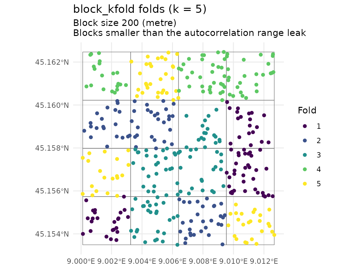

Look at whether any fold is a thin sliver or a single corner. Fold geometry that looks wrong on the map produces a score that is wrong in a way no summary statistic will tell you about.

How wide should a block be?

Wide enough that a test block’s points are uncorrelated with the training points outside it, which makes the autocorrelation range the natural scale.

sac <- estimate_sac_range(pts, "z")
c(range = as.numeric(sac), nugget = sac_nugget(sac))

##       range      nugget 
## 194.0858896   0.1365482

sac_nugget() reads the nugget off the same fitted model. A nugget that is most of the sill says the field has little spatial structure left to leak, and the blocked and random scores will be close.

make_folds(auto_range = TRUE) runs this estimate and uses it as a minimum block size:

fa <- make_folds(pts, k = 5, method = "block_kfold", response_var = "z",
                 auto_range = TRUE, seed = 1)
c(block_size = as.numeric(fa$params$block_size),
  sac_range  = as.numeric(fa$params$sac_range))

## block_size  sac_range 
##   194.0859   194.0859

params$block_size holds the range object itself, so printing it whole also prints the directional summary; as.numeric() above keeps the output to the two numbers.

When the variogram identifies no range, estimate_sac_range() returns NA with the reason attached, auto_range warns that it is falling back to geometric blocks, and you are back to choosing a size yourself. An NA there is a finding about the data. ?estimate_sac_range lists the reasons and what each one means; plot() on the returned object draws the variogram that produced it.

Sizing it by measurement

cv_block_size_sweep() runs the cross-validation at several block sizes and reports the curve, with a random-fold run as the reference.

sw <- cv_block_size_sweep(pts, "z", character(0), fit_fn = knn_fn,
                          k = 4, n_sizes = 5, max_fits = 40,
                          seed = 1, quiet = TRUE)
sw

## Cross-validation RMSE against block size (24 fits, k = 4, sizes in EPSG:32632)
##   estimated autocorrelation range: 194.1
##  block_size       method blocks_used k n_folds_succeeded  value fold_min
##      random random_kfold          NA 4                 4 0.7859   0.7355
##       39.53  block_kfold         291 4                 4 0.7990   0.7449
##       74.33  block_kfold         150 4                 4 0.9137   0.8597
##      139.80  block_kfold          49 4                 4 1.0075   0.8848
##      262.80  block_kfold           9 4                 4 1.0849   0.9119
##      494.10  block_kfold           4 4                 4 1.1296   0.9719
##  fold_max
##    0.8257
##    0.8696
##    0.9891
##    1.1008
##    1.1618
##    1.4184

plot(sw)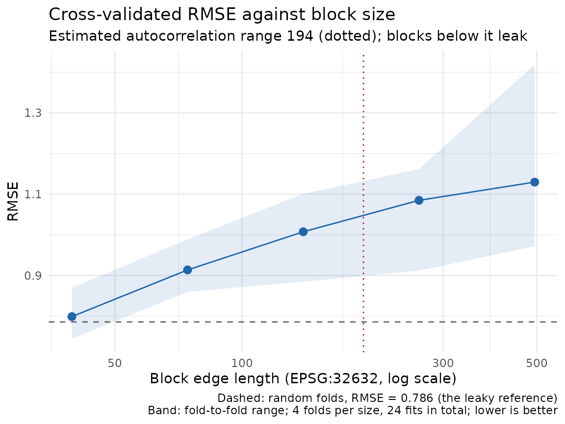

Error climbs away from the random-fold reference as blocks widen, and the estimated range is marked. The height of the climb is what random folds were hiding.

Read the curve up to the range, and watch blocks_used past it. Once blocks_used approaches k, each fold is holding out a large contiguous piece of the study area, and the model is being asked to extrapolate across it. Error keeps rising for a second reason at that point, and the number stops being about leakage.

Reading the result

overall is the pooled score and fold_metrics is one row per fold. plot_cv_metrics() shows the spread, which matters because a pooled RMSE built from one catastrophic fold and four good ones describes neither.

plot_cv_metrics(cv_blocked, metric = "RMSE")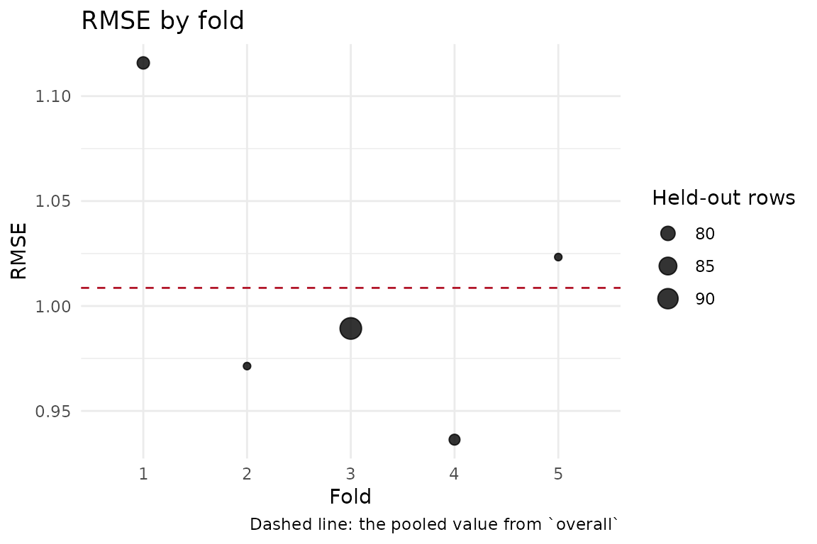

Every row and every fold is accounted for

Four fields say what happened to the data on the way through: n_folds_attempted against n_folds_succeeded, n_dropped (rows the data lost), orphan_rows (rows no fold names) and n_unknown_ids (fold rows the data does not have). On the clean run above nothing went missing:

c(attempted = cv_blocked$n_folds_attempted, succeeded = cv_blocked$n_folds_succeeded,
  dropped = cv_blocked$n_dropped, orphans = length(cv_blocked$orphan_rows))

## attempted succeeded   dropped   orphans 
##         5         5         0         0

So here are two runs where something does.

A learner that fails on one fold:

flaky <- function(train_sf, ...) {
  if (nrow(train_sf) < 320) stop("not enough training rows for this toy learner")
  knn_fit(train_sf, "z", k = 5L)
}
cv_flaky <- cv_spatial(pts, "z", character(0), fit_fn = flaky, folds = fb)

cv_flaky$fold_status

##   fold status                                       message
## 1    1     ok                                              
## 2    2     ok                                              
## 3    3  error not enough training rows for this toy learner
## 4    4     ok                                              
## 5    5     ok

c(attempted = cv_flaky$n_folds_attempted, succeeded = cv_flaky$n_folds_succeeded)

## attempted succeeded 
##         5         4

fold_status names every fold supplied and what became of it, with the error text for the ones that failed. status is one of ok, error, skipped, dropped or worker_error. Before this existed, a partial failure left its causes in console scrollback, which a script or a knitted document does not keep.

Rows the data lost, and rows no fold names:

holed <- pts
holed$z[c(3, 17, 42)] <- NA                       # three rows will be dropped
part  <- make_folds(pts[1:300, ], k = 4, method = "block_kfold", seed = 1)

cv_acc <- cv_spatial(holed, "z", character(0), fit_fn = knn_fn, folds = part)

c(n_dropped     = cv_acc$n_dropped,
  n_orphans     = length(cv_acc$orphan_rows),
  n_unknown_ids = cv_acc$n_unknown_ids)

##     n_dropped     n_orphans n_unknown_ids 
##             3           100             3

n_dropped is how many rows prep_model_data() removed for a missing or non-finite value before any fold was fitted. orphan_rows holds the row IDs no fold names, which here is rows 301 to 400, because the folds were built on the first 300. n_unknown_ids counts the distinct row IDs the folds name that the data does not have, which here is the three rows the NAs removed.

The two mirror each other, and which one is non-zero tells you which way the mismatch runs:

cv_rev <- cv_spatial(pts[1:300, ], "z", character(0), fit_fn = knn_fn, folds = fb)
c(n_orphans = length(cv_rev$orphan_rows), n_unknown_ids = cv_rev$n_unknown_ids)

##     n_orphans n_unknown_ids 
##             0           100

Folds built on more rows than the data has give n_unknown_ids; folds built on fewer give orphan_rows. Both are zero when the folds and the data agree, which is the only case in which the score covers every observation.

Calibration, for a model with intervals

A Bayesian fit predicts an interval, and the question becomes whether the intervals are the width they claim. plot_calibration() draws nominal coverage against realised coverage per fold, from a cv_bayes() result.

cvb <- cv_bayes(pts, "z", character(0), folds = fb)   # needs brms
plot_calibration(cvb)

Points below the diagonal are intervals that are too narrow: a nominal 90 percent interval containing 70 percent of the held-out values is the model reporting more confidence than it has earned. This chunk is not run here, because it needs brms and a Stan toolchain.

Next

vignette("resolution") covers choosing a cell count before any of this. vignette("spatialkit_nc_demo") runs the whole pipeline on real boundaries. ?make_folds documents every scheme and its arguments, ?cv_spatial the return value in full, and ?cv_block_size_sweep the fit budget that max_fits caps.