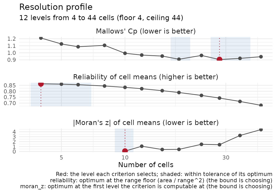
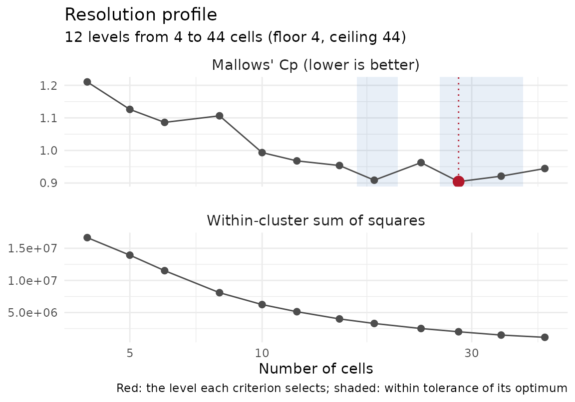
The criteria of a resolution_profile() against the number of
cells, one panel per criterion on a shared x axis, with the level each
criterion selects marked and the region over which it is within tol
of its optimum shaded. That shaded band is the flat region
select_resolution() reports. A criterion whose optimum sits
at an end of the levels it was scored at is captioned with which bound that
is (the support ceiling, the range floor, the ladder's own end, or the
first level the criterion is computable at), because there the bound is
choosing, not the criterion. A criterion that is NA at every
level is left out with a log line rather than drawn empty.
Usage
# S3 method for class 'resolution_profile'
plot(x, criteria = NULL, tol = 0.02, ...)
Arguments
- x
A
resolution_profile.- criteria
Character vector of criteria to draw, any of
"cp","reliability","elbow","moran_z","wss". Default: every one of the four selectable criteria that is finite at some level."wss"is the raw curve behind"elbow"and has no selected point.- tol
Passed to
select_resolution()for the flat region.- ...
Ignored.
Examples
if (requireNamespace("gstat", quietly = TRUE) &&
    requireNamespace("ggplot2", quietly = TRUE)) {
  library(sf)
  # The same field as ?resolution_profile: an exponential covariance with
  # range parameter 200 and a nugget of 0.6 on a unit sill.
  set.seed(4)
  n <- 400
  xy <- data.frame(x = 5e5 + runif(n, 0, 1000), y = 5e6 + runif(n, 0, 1000))
  D  <- as.matrix(dist(xy))
  xy$z <- as.numeric(t(chol(exp(-D / 200) + diag(0.6, n))) %*% rnorm(n))
  pts <- st_as_sf(xy, coords = c("x", "y"), crs = 32632)
  prof <- resolution_profile(pts, response_var = "z", n_levels = 12)
  print(plot(prof))                     # one panel per criterion it scored: no
                                        # elbow on these uniform points
  plot(prof, criteria = c("cp", "wss")) # Cp beside the raw WSS curve
}