Plot an estimated spatial autocorrelation range

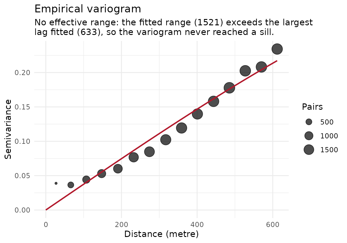
Draws the empirical variogram that estimate_sac_range() attaches to its result, with the fitted model and the effective range overlaid where a range was identified, and a subtitle saying why not where it was not. A variogram that never reaches a sill, or that has no spatial structure at the lags resolved, is the single most useful thing to see when a range comes back NA, so those cases are drawn rather than refused.

Usage

# S3 method for class 'sac_range'
plot(x, ...)

Arguments

x

An object of class sac_range, as returned by estimate_sac_range().

...

Ignored.

Value

A ggplot object.

Details

Nothing is recomputed: the plot reads the variogram, variogram_model, crs, directional and anisotropy_used attributes the estimate already carries. The distance axis is in the units of the CRS the variogram was actually fitted in, which estimate_sac_range() may have chosen itself for lon/lat input.

See also

plot.spatial_fit(type = "variogram"), which draws the same picture for a fitted model's residuals.

Other plotting: plot.aoa(), plot.block_size_sweep(), plot.feature_selection(), plot.gwr_model_selection(), plot.resolution_profile(), plot.spatial_fit(), plot_calibration(), plot_cv_metrics(), plot_folds()

Examples

if (requireNamespace("gstat", quietly = TRUE) &&
    requireNamespace("ggplot2", quietly = TRUE)) {
  library(sf)
  # An exponential field with range parameter 150 (effective range about
  # 450 m) and a nugget of half the sill, so the fitted model, the nugget
  # and the range line all have something to show.
  set.seed(3)
  n <- 250
  xy <- data.frame(x = 5e5 + runif(n, 0, 1000), y = 5e6 + runif(n, 0, 1000))
  D  <- as.matrix(dist(xy))
  xy$z <- as.numeric(t(chol(exp(-D / 150) + diag(0.5, n))) %*% rnorm(n))
  pts <- st_as_sf(xy, coords = c("x", "y"), crs = 32632)
  r <- estimate_sac_range(pts, response_var = "z")
  plot(r)

  # A field whose variogram never reaches a sill: the plot still draws it,
  # and the subtitle says why no range is marked.
  xy$trend <- sin(xy$x / 400) + rnorm(n, sd = 0.2)
  r2 <- estimate_sac_range(st_as_sf(xy, coords = c("x", "y"), crs = 32632),
                           response_var = "trend")
  plot(r2)
}