Plot a fitted spatial model

Diagnostic plots for a spatial_fit. The package previously shipped print() and summary() methods but no plot(), so the checks most likely to reveal a problem (is there structure left in the residuals, and where is it) had to be written by hand each time.

Usage

# S3 method for class 'spatial_fit'
plot(
  x,
  type = c("residuals", "observed_predicted", "variogram", "coefficients"),
  response = TRUE,
  term = NULL,
  mask = TRUE,
  ...
)

Arguments

x

A spatial_fit. The residuals drawn are residuals(x); for a custom subclass with no residuals() method (optional, see new_spatial_fit()) they are the response minus fitted(x), which is what the built-in backends' methods return.

type

One of:

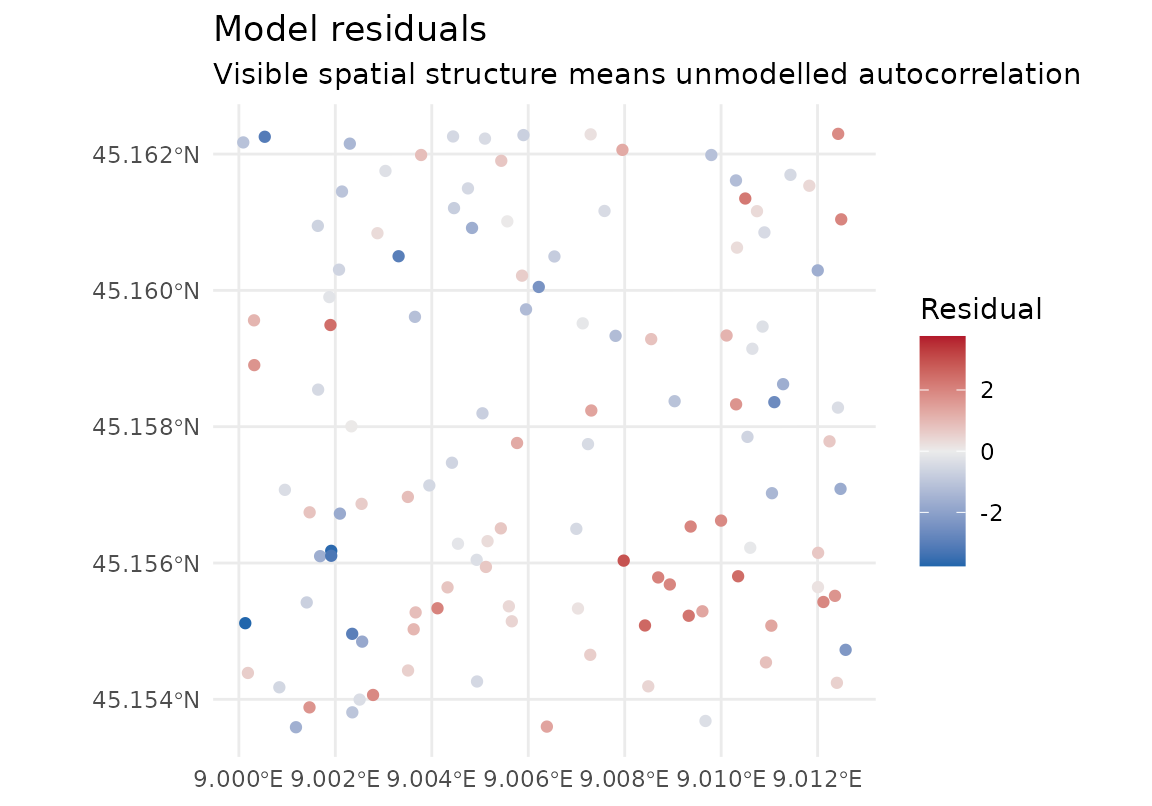
"residuals"

Residuals mapped at the training locations. Spatial structure here is the signal that the model has not captured the autocorrelation.

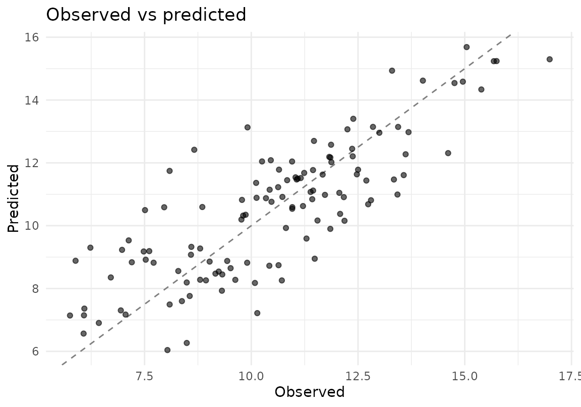
"observed_predicted"

Observed against fitted, with a 1:1 reference line.

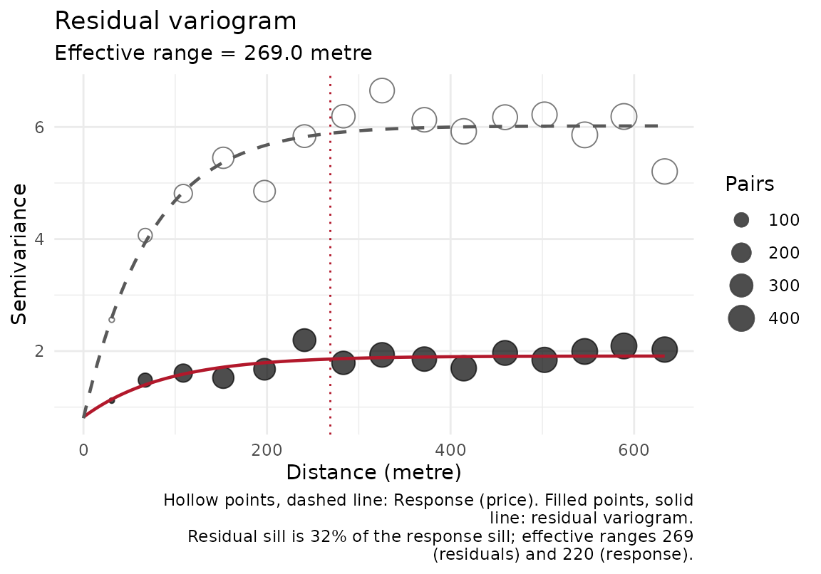
"variogram"

Empirical variogram of the residuals with the fitted model overlaid, so the fit can be judged rather than trusted, and (unless response = FALSE) the variogram of the response itself on the same points and lags, drawn hollow with a dashed fit. The gap between the two curves is the spatial structure the model absorbed: a residual sill well below the response sill means most of it, two curves that coincide mean none. When both effective ranges were identified over the same point pairs the caption gives the residual sill as a share of the response sill and the two ranges; when either variogram has no identified range, or the two are not over the same pairs, the caption says so and compares nothing: a sill the data never reached is not a number to divide by, and one direction's sill is not comparable with all directions'. The residual range is expected to come out shorter and the residual sill lower even when the model is right, because residuals of a fitted trend understate the variogram (see estimate_sac_range(), "Detrending and the residual-variogram bias"). The distance axis is labelled in the units of the CRS the variogram was actually fitted in, which is not necessarily the fit's own CRS (lon/lat data are projected first). Each curve is the variogram estimate_sac_range() returns for its variable: all point pairs, or, when the all-pairs fit was unusable, the widest of four directions, which is named with its azimuth (in the title for the residuals, in the caption for the response). A fit that identified no range says why in the subtitle, since the overlaid model line is then not a fit to believe. Requires 'gstat'.

"coefficients"

For a GWR fit only: the local coefficient of one term mapped at the training locations, which is the reason to fit GWR at all. Locations where the local design is collinear for that term are drawn hollow and grey (mask = TRUE): for a slope, where the kernel-weighted window's slope condition index (cn_slopes, predictors centred in the window) is above 30 or the window is singular, or where the index with the intercept (cn) is above 1e6; for the Intercept, where cn is above 30 (a predictor far from 0 against its local spread makes the local intercept an extrapolation). They are masked because the smooth surface a naive map draws over them is the picture of an unstable estimate, not of a relationship; the subtitle counts them. The condition indices are the fit's info$local_collinearity, computed for every location when the model was fitted. A diverging scale centred on zero is used when the coefficient changes sign, otherwise a sequential one.

response

Logical, default TRUE: for type = "variogram", overlay the response's own variogram. Ignored by the other types.

term

For type = "coefficients": which local coefficient to map, one of the names coef(x) returns. Default NULL: the first predictor. Ignored by the other types.

mask

For type = "coefficients": whether to draw locations whose local design is collinear for that term (see type = "coefficients") as hollow grey points instead of colouring them by a coefficient that is not to be believed there. Default TRUE. Locations whose coefficient is non-finite are masked either way.

...

Ignored.

Value

A ggplot object.

See also

coef.gwr_fit() for the coefficients themselves.

Other plotting: plot.aoa(), plot.block_size_sweep(), plot.feature_selection(), plot.gwr_model_selection(), plot.resolution_profile(), plot.sac_range(), plot_calibration(), plot_cv_metrics(), plot_folds()

Examples

# Works on any spatial_fit; a forest keeps the example free of the optional
# GWR/Stan backends.
if (requireNamespace("ranger", quietly = TRUE) &&
    requireNamespace("ggplot2", quietly = TRUE)) {
  library(sf)
  # price depends on elevation, which the forest sees, and on a spatially
  # correlated field it does not: that field is what the residual plots
  # are there to find.
  set.seed(2)
  n <- 120
  xy <- data.frame(x = 5e5 + runif(n, 0, 1000), y = 5e6 + runif(n, 0, 1000),
                   elev = rnorm(n))
  D  <- as.matrix(dist(xy[, c("x", "y")]))
  xy$price <- 10 + 2 * xy$elev +
    as.numeric(t(chol(exp(-D / 100) + diag(0.3, n))) %*% rnorm(n))
  pts <- st_as_sf(xy, coords = c("x", "y"), crs = 32632)
  fit <- fit_rf_model(pts, "price", "elev", num_trees = 100, seed = 1)
  # print() each one: inside a braced block only the last value is drawn.
  print(plot(fit, type = "residuals"))          # structure left in the residuals
  print(plot(fit, type = "observed_predicted"))
  if (requireNamespace("gstat", quietly = TRUE))
    plot(fit, type = "variogram")   # residual and response variograms compared
}