ANCOVA: comparing groups at the same value of a covariate

library(anovakit)

anova_ancova() compares the mean of a numeric response across groups while adjusting for one or more numeric covariates. Use it when something you measured before the groups could differ – a baseline score, a starting weight – also predicts the outcome: adjusting for it removes that source of noise and compares the groups at the same value of the covariate. With no covariate, use anova_welch() or anova_glm(); with several responses, anova_manova() accepts covariates too. The decision guide covers the choice in more detail.

The data

MASS::anorexia records the weight (in pounds) of 72 young women with anorexia before and after a period of treatment: cognitive behavioural treatment (CBT), family treatment (FT) or a control condition (Cont).

an <- MASS::anorexia
head(an)
#>   Treat Prewt Postwt
#> 1  Cont  80.7   80.2
#> 2  Cont  89.4   80.1
#> 3  Cont  91.8   86.4
#> 4  Cont  74.0   86.3
#> 5  Cont  78.1   76.1
#> 6  Cont  88.3   78.1
table(an$Treat)
#> 
#>  CBT Cont   FT 
#>   29   26   17
aggregate(cbind(Prewt, Postwt) ~ Treat, data = an, FUN = mean)
#>   Treat    Prewt   Postwt
#> 1   CBT 82.68966 85.69655
#> 2  Cont 81.55769 81.10769
#> 3    FT 83.22941 90.49412

The groups start at slightly different weights, and a patient’s weight afterwards depends partly on where she started (the correlation between the two is 0.33). The question an ANCOVA answers is: for patients of the same starting weight, does the treatment make a difference to the weight afterwards? Postwt is the response, Treat the grouping variable and Prewt the covariate.

Fitting the model

Columns are named as character strings: the response, then the grouping variable(s), then the covariate(s).

fit <- anova_ancova(an, "Postwt", "Treat", "Prewt")
fit
#> Analysis of covariance (Type III) 
#> ---------------------------------
#> Call: anova_ancova(data = an, response = "Postwt", groups = "Treat", covariates = "Prewt")
#> Observations used: 72
#> 
#> Omnibus test (Type III, F)
#>          term sum_sq df statistic   p_value
#> 1       Prewt  503.4  1    11.680 0.0010866
#> 2       Treat  785.1  2     9.107 0.0003215
#> 3 Prewt:Treat  466.5  2     5.411 0.0066656
#> 4   Residuals 2845.0 66        NA        NA
#> 
#> Notes
#>   - Covariate(s) mean-centred before fitting (Prewt: 82.41), so the intercept and the Type III group row refer to the covariate mean rather than to covariate = 0. $emmeans are evaluated at the covariate mean either way.
#>   - Slopes differ across groups (p = 0.006666), so the covariate-by-group interaction was retained. The group row of the ANOVA table is then a comparison at the covariate mean, not a constant adjusted difference: read $simple_slopes and $emmeans instead.
#>   - The model was chosen by a test on these same data, and the p-values below do not allow for that choice: given that the test retained the slope terms, they can be noticeably too small, especially in small samples. Setting force_interaction = TRUE in advance avoids the selection step; the group row is then a valid comparison at the covariate mean whether or not the slopes differ.
#> 
#> Plots available: residuals, qq, covariate, emmeans
#>   (use plot(x, which = "residuals"))

Reading the printout from the top:

The method line says the tests use Type III sums of squares (the default type = "III", fitted under sum-to-zero contrasts).
Observations used is the number of rows in $data_used. Rows with a missing value in any analysed column are dropped and counted in $n_removed; there are none here.
The omnibus table has a Prewt:Treat row because the function fitted two candidate models and a homogeneity-of-slopes test chose the one with a separate slope for each group (see the next section).
The notes say what the function decided and why. Read them on every fit; they are discussed below.
Plots available lists the ggplot2 objects in $plots.

summary(fit) prints all of this and then the assumption checks, effect sizes, marginal means, pairwise comparisons, the slopes test and the per-group slopes. The rest of this article takes those components one at a time.

The homogeneity-of-slopes test

Classical ANCOVA assumes that the covariate has the same slope in every group, so that the groups differ by a constant amount whatever the covariate value. anova_ancova() checks this before anything else. It fits two candidate models – the covariate entered additively, and the same model plus the product of the covariate with the grouping terms – and compares them with one nested F test:

fit$slopes_test
#>                                   comparison df statistic     p_value
#> 1 additive vs covariate-by-group interaction  2  5.411231 0.006665591
#>   homogeneous
#> 1       FALSE

Here the test rejects (p = 0.00667), so homogeneous is FALSE and the interaction model was fitted. Both candidates are kept, so the one not chosen is still available, and the comparison can be reproduced from them:

deparse(formula(fit$model_additive))
#> [1] "Postwt ~ Prewt + Treat"
deparse(formula(fit$model_interaction))
#> [1] "Postwt ~ Prewt + Treat + Prewt:Treat"
anova(fit$model_additive, fit$model_interaction)
#> Analysis of Variance Table
#> 
#> Model 1: Postwt ~ Prewt + Treat
#> Model 2: Postwt ~ Prewt + Treat + Prewt:Treat
#>   Res.Df    RSS Df Sum of Sq      F   Pr(>F)   
#> 1     68 3311.3                                
#> 2     66 2844.8  2    466.48 5.4112 0.006666 **
#> ---
#> Signif. codes:  0 '***' 0.001 '**' 0.01 '*' 0.05 '.' 0.1 ' ' 1

When the slopes differ, the thing to read is the slope in each group, $simple_slopes (from emmeans::emtrends()):

print(fit$simple_slopes[, c("Treat", "slope", "se", "conf_low", "conf_high",
                            "p_value")], digits = 3)
#>   Treat  slope    se conf_low conf_high p_value
#> 1   CBT  0.848 0.256    0.337     1.359 0.00151
#> 2  Cont -0.134 0.230   -0.594     0.325 0.56173
#> 3    FT  0.909 0.327    0.256     1.562 0.00709

In both active treatments a heavier start goes with a heavier finish (about 0.85 and 0.91 lb per lb), but in the control group there is essentially no relation (-0.13, with an interval that spans zero). The treatment effect is therefore not one number: it depends on the starting weight. $simple_slopes is NULL whenever the additive model is used, because there is then only one slope.

Why `force_interaction` exists

Letting a test on the same data choose the model has a cost in both directions, and the notes say so. When the test retains the interaction, as here, the p-values that follow do not allow for that choice and can be too small. When the slopes really differ but the test misses it, the additive model’s adjusted comparisons are biased by the slope difference times the difference in covariate means – which averages out when groups are randomised, but not otherwise. The help page (?anova_ancova) reports simulations of how often that second case rejects a true null hypothesis.

force_interaction removes the selection step. Decide in advance:

force_interaction = TRUE always fits the separate-slopes model. With centred covariates and Type III tests, the group row is then a valid comparison of the groups at the covariate mean whether or not the slopes differ. This is the safer choice when the groups were not randomised.
force_interaction = FALSE always fits the additive model.
NULL (the default) lets the slopes test decide, at level homogeneity_alpha (0.05 by default).

fixed <- anova_ancova(an, "Postwt", "Treat", "Prewt", force_interaction = TRUE,
                      plots = FALSE)
all.equal(fixed$anova, fit$anova)
#> [1] TRUE
fixed$notes[2]
#> [1] "The covariate-by-group interaction was fitted because force_interaction = TRUE; the homogeneity-of-slopes test itself gave p = 0.006666. The group row of the ANOVA table is then a comparison at the covariate mean, not a constant adjusted difference: read $simple_slopes and $emmeans instead."

The model and the table are the same as before – the test happened to choose the same model – but the notes now say the choice was yours, and the warning about selection is gone.

The omnibus test

fit$anova
#>          term    sum_sq df statistic      p_value
#> 1       Prewt  503.4196  1 11.679513 0.0010866494
#> 2       Treat  785.1051  2  9.107357 0.0003214744
#> 3 Prewt:Treat  466.4783  2  5.411231 0.0066655907
#> 4   Residuals 2844.7843 66        NA           NA

Each row is a term of the model:

sum_sq is its Type III sum of squares: what the term adds when every other term is already in the model. Residuals is the error sum of squares.
df is its degrees of freedom (a three-level factor has 2).
statistic is the F ratio, the term’s mean square over the residual mean square, and p_value its upper-tail probability on df and the residual degrees of freedom.

The Treat row is the one most people want, and in this model it needs care. Because the covariate is centred and the slopes are separate, it compares the groups at the mean starting weight (82.4 lb). It is not a constant treatment effect, since there is none when the slopes differ. Prewt tests the covariate’s slope averaged over the groups, and Prewt:Treat is the slope difference the homogeneity test found (with the same F and p-value).

Effect sizes

fit$effect_sizes
#>          term df   sum_sq partial_eta_sq partial_omega_sq
#> 1       Prewt  1 503.4196      0.1503551        0.1291676
#> 2       Treat  2 785.1051      0.2162890        0.1838096
#> 3 Prewt:Treat  2 466.4783      0.1408763        0.1091585

partial_eta_sq is the term’s sum of squares over itself plus the residual sum of squares: the share of the variation not explained by the other terms that this term explains. partial_omega_sq corrects that for the bias of a sample estimate and is the better estimate of the population value; it is floored at 0 (with a note) when a term explains less than chance would. Both are partial measures, each with its own denominator, and Type III sums of squares do not add up to the total, so do not add the rows together. Neither comes with an interval.

Covariate centring

Every covariate is mean-centred before fitting (center_covariates = TRUE). The means subtracted are in $covariate_means, and $data_used holds the centred values:

fit$covariate_means
#>    Prewt 
#> 82.40833
head(fit$data_used, 3)
#>   Postwt Treat     Prewt .cell
#> 1   80.2  Cont -1.708333  Cont
#> 2   80.1  Cont  6.991667  Cont
#> 3   86.4  Cont  9.391667  Cont

What centring changes depends on the model. It always moves the intercept. When the covariate-by-group terms are in the model and type = "III", it also moves the group row, because that row then tests the groups at covariate = 0. Without centring, zero pounds is a starting weight none of these patients had:

unc <- anova_ancova(an, "Postwt", "Treat", "Prewt", center_covariates = FALSE,
                    plots = FALSE)
data.frame(term = fit$anova$term,
           p_centred = fit$anova$p_value,
           p_uncentred = unc$anova$p_value)
#>          term    p_centred p_uncentred
#> 1       Prewt 0.0010866494 0.001086649
#> 2       Treat 0.0003214744 0.012945287
#> 3 Prewt:Treat 0.0066655907 0.006665591
#> 4   Residuals           NA          NA
all.equal(fit$emmeans, unc$emmeans)
#> [1] TRUE

Only the Treat row changed. The covariate row, the interaction row and the adjusted means are identical, because $emmeans, $posthoc and $simple_slopes are always evaluated with every covariate at its mean. In the additive model, and under Type II, centring does not change the group row at all. Set center_covariates = FALSE only if the covariate’s own zero is the point you want the intercept to describe; the notes of unc explain what it did.

Marginal means and comparisons

fit$emmeans
#>   Treat estimate       se df conf_low conf_high
#> 1   CBT 85.45800 1.221267 66 83.01966  87.89633
#> 2  Cont 80.99355 1.302345 66 78.39333  83.59377
#> 3    FT 89.74757 1.614813 66 86.52349  92.97165

These are covariate-adjusted means: the predicted post-treatment weight in each group for a patient starting at the mean weight of 82.41 lb. They differ from the raw means above because the groups did not start at exactly that weight.

print(fit$posthoc[, c("contrast", "estimate", "conf_low", "conf_high",
                      "p_value", "p_adjusted", "adjustment")], digits = 3)
#>     contrast estimate conf_low conf_high  p_value p_adjusted adjustment
#> 1 CBT - Cont     4.46    0.184     8.745 1.49e-02   0.039034      tukey
#> 2   CBT - FT    -4.29   -9.144     0.565 3.79e-02   0.093792      tukey
#> 3  Cont - FT    -8.75  -13.728    -3.780 7.63e-05   0.000223      tukey

p_value is the unadjusted p-value of each comparison; p_adjusted is adjusted for the three comparisons by the method in adjustment (Tukey by default), and the intervals are adjusted to match. Report p_adjusted when you are looking at all pairs. adjust takes any of the methods listed on the help page, for example adjust = "holm"; "none" makes the two columns equal.

holm <- anova_ancova(an, "Postwt", "Treat", "Prewt", adjust = "holm",
                     plots = FALSE)
print(holm$posthoc[, c("contrast", "p_value", "p_adjusted")], digits = 3)
#>     contrast  p_value p_adjusted
#> 1 CBT - Cont 1.49e-02   0.029782
#> 2   CBT - FT 3.79e-02   0.037884
#> 3  Cont - FT 7.63e-05   0.000229

The emmeans grid itself is in $emmeans_object, for any contrast the wrapper does not compute (give level = when you summarise it; see Working with results).

What the adjustment buys

Compare this with two analyses that ignore the starting weight in different ways. anova_welch() compares the raw post-treatment weights; an ANOVA on the change scores (Postwt - Prewt) assumes that each pound of starting weight carries over one for one, a slope of exactly 1.

welch <- anova_welch(an, "Postwt", "Treat", plots = FALSE)
print(welch$posthoc[, c("group1", "group2", "difference", "p_adjusted")],
      digits = 3)
#>   group1 group2 difference p_adjusted
#> 1    CBT   Cont       4.59    0.02938
#> 2    CBT     FT      -4.80    0.07129
#> 3   Cont     FT      -9.39    0.00117

an$change <- an$Postwt - an$Prewt
chg <- anova_glm(an, "change", "Treat", plots = FALSE)
print(chg$posthoc[, c("contrast", "estimate", "p_adjusted")], digits = 3)
#>     contrast estimate p_adjusted
#> 1 CBT - Cont     3.46    0.21244
#> 2   CBT - FT    -4.26    0.16075
#> 3  Cont - FT    -7.71    0.00451

All three find that family treatment beats the control, but they answer different questions. Welch’s test ignores the starting weight altogether: its CBT-control difference of 4.59 lb makes no allowance for the 1.13 lb by which the CBT group started heavier, and the variation the starting weight explains stays in the error. The change-score analysis imposes a slope of 1, which the simple slopes above show no group has, and with it the CBT-control comparison weakens to adjusted p = 0.21, against 0.039 in the ANCOVA. ANCOVA estimates the slope from the data instead, which is why it is usually the better choice for a pre-post design.

Checking assumptions

names(fit$assumptions)
#> [1] "normality" "levene"    "slopes"
fit$assumptions$normality
#> 
#>  Shapiro-Wilk normality test
#> 
#> data:  x
#> W = 0.97938, p-value = 0.2846
fit$assumptions$levene
#>   df1 df2 statistic   p_value
#> 1   2  69   1.02573 0.3639361

normality is a Shapiro-Wilk test on the model residuals. It tests the assumption that the errors are normal; a small p-value in a small sample deserves a look at the Q-Q plot, while in a large sample the test flags departures too small to matter. Here W = 0.979 and p = 0.28.
levene is Levene’s test (on absolute deviations from the medians) of the residuals across the groups (the cells, with several grouping variables). A rejection means the pooled residual variance is not a fair summary; the note it triggers suggests vcov_type = "HC3", shown below. Here p = 0.36.
slopes is the homogeneity-of-slopes test, the same table as $slopes_test.

A covariate that is constant, constant within every group, or an exact linear combination of the groups and the other covariates is refused with an error rather than fitted, since there is nothing to adjust for. The diagnostics article covers the checks across the package.

Plots

Every plot is a ggplot2 object in $plots; plot(fit, "name") returns one, and you can add layers or themes to it with + (see Plots and visual customisation).

Residuals against fitted values

plot(fit, "residuals")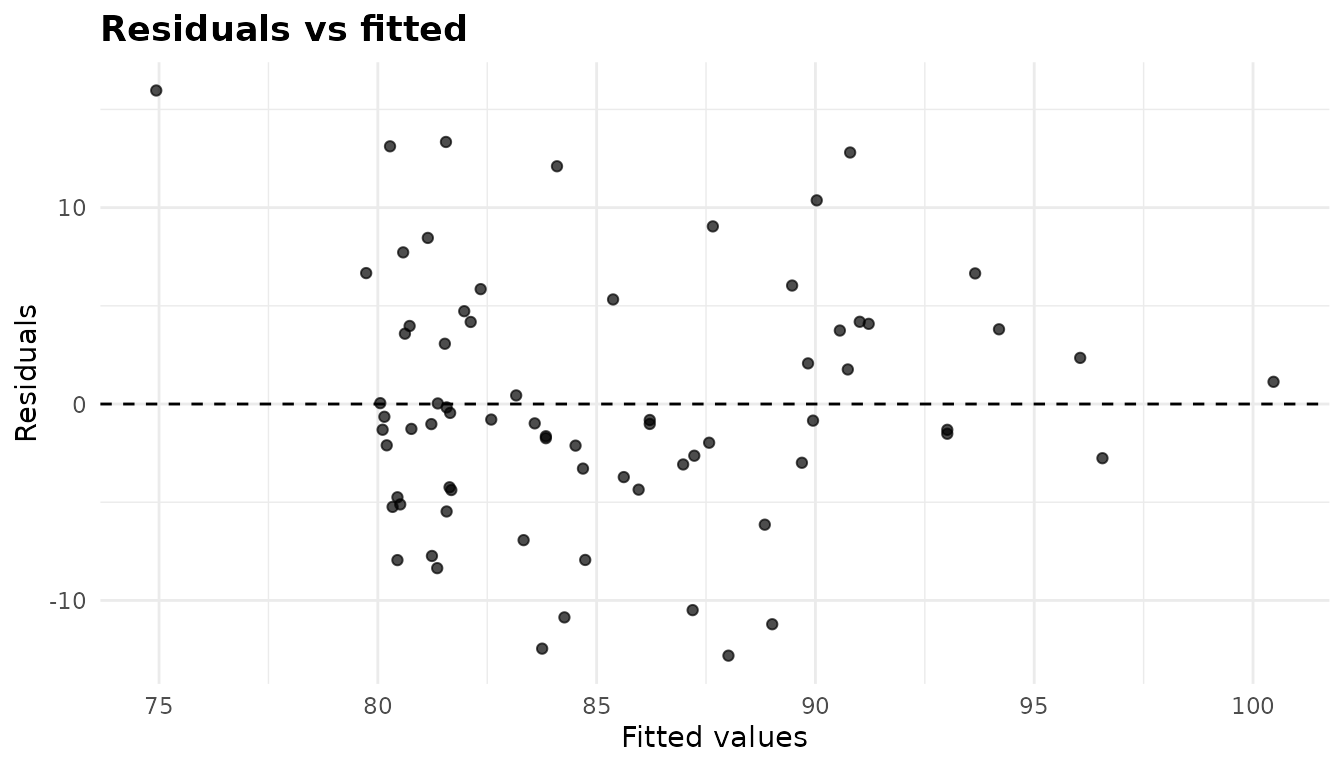

What to look for: an even band around zero. A funnel (spread growing with the fitted value) points to unequal variances; a curve points to a covariate relation that is not linear. Here there is neither. The tight column of points at fitted values of about 80 to 82 lb is the control group: with a nearly flat slope, its fitted values hardly vary.

Normal Q-Q plot

plot(fit, "qq")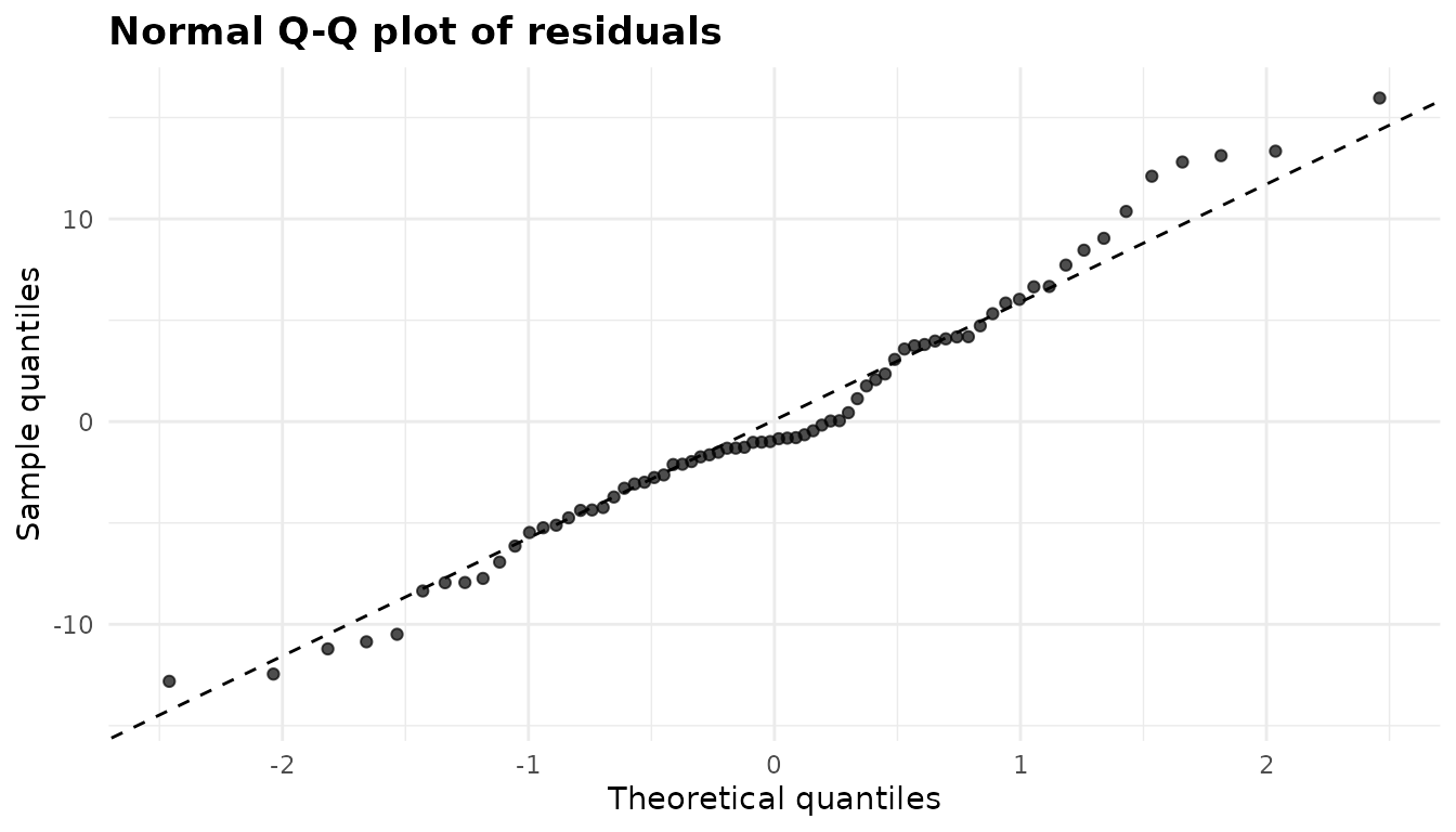

What to look for: points close to the dashed line. Systematic bends at the ends mean heavy or light tails; a single point far off it is an outlier worth checking in the data. These residuals follow the line with a mild S-shape, which is in keeping with the Shapiro-Wilk test above.

The covariate plot

plot(fit, "covariate")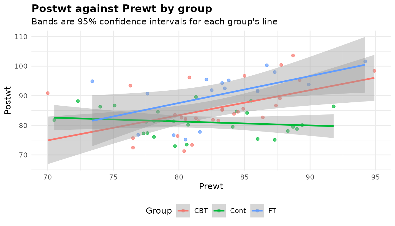

This is the plot to look at first in any ANCOVA. It shows the response against the covariate on its original scale, with a separate least-squares line and confidence band for each group (the bands use conf_level). The lines are each group’s own fit, drawn whichever model was chosen, so they show you directly whether parallel lines are a fair description. Here they are not: the control group’s line is almost flat while the two treatment lines rise. Look too at whether the groups cover the same range of the covariate – adjusted means for a group observed only at one end are extrapolations, and $notes names such a group. With several covariates there is one plot per covariate, named covariate_<name>.

Adjusted means

plot(fit, "emmeans")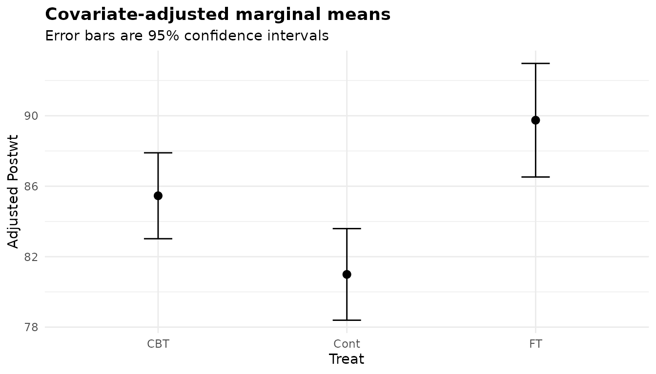

The covariate-adjusted means from $emmeans with their confidence intervals. With a separate-slopes model, remember that these are the group means at one starting weight; the covariate plot shows how the gaps change away from it.

Options worth knowing

Robust tests with `vcov_type`

vcov_type = "HC3" (or "HC0" to "HC4", which need the sandwich package) replaces the model-based covariance with a heteroscedasticity-consistent one.

rob <- anova_ancova(an, "Postwt", "Treat", "Prewt", force_interaction = TRUE,
                    vcov_type = "HC3", plots = FALSE)
rob$anova
#>          term df statistic     p_value
#> 1       Prewt  1  4.733147 0.033172900
#> 2       Treat  2  7.529746 0.001133501
#> 3 Prewt:Treat  2  3.211929 0.046650376
#> 4   Residuals 66        NA          NA
attr(rob$anova, "statistic")
#> [1] "Wald F with HC3 covariance"
data.frame(Treat = fit$emmeans$Treat, se_model = fit$emmeans$se,
           se_HC3 = rob$emmeans$se)
#>   Treat se_model   se_HC3
#> 1   CBT 1.221267 1.572187
#> 2  Cont 1.302345 0.983944
#> 3    FT 1.614813 2.317611

The F tests in $anova are now Wald F tests built from the robust covariance (through car::Anova(vcov. = )), on the model’s residual degrees of freedom, so the table has no sums of squares, and its statistic attribute (which print() shows in the heading) says so. The same covariance reaches $emmeans, $posthoc and $simple_slopes: the control group’s standard error shrinks and the family-treatment group’s grows, reflecting their different residual spreads. Two things do not change: $effect_sizes still come from the model-based sums of squares, and the homogeneity-of-slopes test stays the model-based F test. The notes of rob say both.

Several grouping variables: `interaction`

With two or more grouping variables, the default interaction = TRUE fits their full factorial, which is what a factorial ANCOVA is. MASS::birthwt has birth weights (grams) by the mother’s race and smoking status, with the mother’s weight (pounds) as a covariate.

bw <- MASS::birthwt
bw$race <- factor(bw$race, labels = c("white", "black", "other"))
bw$smoke <- factor(bw$smoke, labels = c("no", "yes"))

two <- anova_ancova(bw, "bwt", c("race", "smoke"), "lwt", plots = FALSE)
two$anova
#>         term   sum_sq  df statistic    p_value
#> 1        lwt  2001912   1  4.362005 0.03814039
#> 2       race  5997349   2  6.533870 0.00181811
#> 3      smoke  2993902   1  6.523471 0.01146521
#> 4 race:smoke  1634954   2  1.781216 0.17135671
#> 5  Residuals 83527636 182        NA         NA
two$slopes_test
#>                                   comparison df statistic   p_value homogeneous
#> 1 additive vs covariate-by-group interaction  5 0.6308707 0.6764194        TRUE

The slopes test now allows a separate slope in every cell (5 extra degrees of freedom) and finds no evidence against a common one, so the additive-covariate model is used. $emmeans and $posthoc compare the six cells:

print(two$emmeans, digits = 4)
#>    race smoke estimate     se  df conf_low conf_high
#> 1 white    no     3397 103.29 182     3193      3600
#> 2 black    no     2784 172.65 182     2444      3125
#> 3 other    no     2854  93.15 182     2670      3038
#> 4 white   yes     2839  94.14 182     2654      3025
#> 5 black   yes     2458 215.34 182     2033      2883
#> 6 other   yes     2778 195.82 182     2392      3164

With interaction = FALSE the grouping variables enter additively, and the means and comparisons are reported for each factor separately, averaged over the other, with a term column; each factor is its own multiplicity family.

add <- anova_ancova(bw, "bwt", c("race", "smoke"), "lwt", interaction = FALSE,
                    plots = FALSE)
print(add$posthoc[, c("term", "contrast", "estimate", "p_adjusted")],
      digits = 3)
#>    term      contrast estimate p_adjusted
#> 1  race white - black      504   0.003416
#> 2  race white - other      395   0.002788
#> 3  race black - other     -109   0.788885
#> 4 smoke      no - yes      400   0.000302

A whole number keeps interactions up to that order. The notes of both fits carry one more message worth reading:

two$notes[3]
#> [1] "The covariate means differ between groups (largest difference: lwt 1.03 pooled within-group SDs). With the slopes assumed equal, any real difference in slopes biases the adjusted comparisons by the slope difference times the covariate-mean difference, and the homogeneity-of-slopes test often lacks the power to detect a difference large enough to matter, so the group row and $posthoc can reject far more often than their nominal level. force_interaction = TRUE does not assume equal slopes."

The mothers’ mean weights differ between the cells by up to 1.03 pooled within-group SDs, so a slope difference the test missed would bias the comparisons. Since smoking and race were not randomised, this is the situation where force_interaction = TRUE is the safer choice.

The rest

type = "II" gives Type II sums of squares, where each term is adjusted for every other term that does not contain it. Under Type II the group row is the same whether or not the covariate is centred.
conf_level sets the level of every interval: the marginal means, the comparisons, the simple slopes and the bands of the covariate plot.
homogeneity_alpha is the level of the slopes test (default 0.05).
posthoc = FALSE skips the pairwise comparisons, which is worth doing when there are many cells; a note records it.
plots = FALSE skips building the plots, which saves time in a loop.

What the notes say

fit$notes
#> [1] "Covariate(s) mean-centred before fitting (Prewt: 82.41), so the intercept and the Type III group row refer to the covariate mean rather than to covariate = 0. $emmeans are evaluated at the covariate mean either way."                                                                                                                                                                     
#> [2] "Slopes differ across groups (p = 0.006666), so the covariate-by-group interaction was retained. The group row of the ANOVA table is then a comparison at the covariate mean, not a constant adjusted difference: read $simple_slopes and $emmeans instead."                                                                                                                                  
#> [3] "The model was chosen by a test on these same data, and the p-values below do not allow for that choice: given that the test retained the slope terms, they can be noticeably too small, especially in small samples. Setting force_interaction = TRUE in advance avoids the selection step; the group row is then a valid comparison at the covariate mean whether or not the slopes differ."

The covariate was centred at its mean, and so the Type III group row compares the groups at Prewt = 82.41 rather than at 0. The marginal means are at the mean either way.
The slopes test rejected, so the interaction model was kept, and the group row is a comparison at one point on the covariate: read $simple_slopes and $emmeans.
The model was chosen by a test on the same data, so the p-values do not account for that choice. force_interaction = TRUE, decided in advance, avoids it.

Other notes appear when they apply: an imbalance warning when the additive model is used and the covariate means differ between groups by more than half a pooled within-group SD (as in the birth-weight example), an extrapolation warning when the covariate mean lies outside a group’s observed range, a Levene rejection, dropped rows, and anything lm(), car or emmeans said while the model was being fitted.

Reporting the result

Post-treatment weight was analysed by ANCOVA with pre-treatment weight (centred at its mean, 82.4 lb) as the covariate. The slope of pre-treatment weight differed between treatments, F(2, 66) = 5.41, p = 0.0067: it was 0.85 for CBT, 0.91 for family treatment and -0.13 for the control group, so the model kept separate slopes. At the mean pre-treatment weight, post-treatment weight differed between treatments, F(2, 66) = 9.11, p < 0.001, partial η² = 0.22. Adjusted means were 89.7 lb (family treatment), 85.5 lb (CBT) and 81.0 lb (control). Family treatment exceeded the control by 8.8 lb (Tukey-adjusted p < 0.001) and CBT exceeded it by 4.5 lb (p = 0.039); the two treatments did not differ clearly (p = 0.094). Because the model was chosen by a test on the same data, these p-values may be somewhat too small.