Repeated measures ANOVA: the same subjects under several conditions

library(anovakit)

anova_rm() fits a repeated measures ANOVA, in which every subject is measured in every cell of one or more within-subject factors, optionally with between-subject factors that split the subjects into groups. It takes data in long format (one row per subject per cell), fits the model with afex::aov_ez() and so needs the afex package. If each subject contributes a single observation, the groups are independent and anova_welch() or anova_glm() is the right tool; for a before-and-after design where the question is about the “after”, anova_ancova() with the baseline as a covariate is often better. The decision guide has more.

The data

afex::obk.long is the long form of a contrived data set from O’Brien and Kaiser (1985): 16 subjects in three treatments (control, A, B), of both genders, each measured at a pre-test, a post-test and a follow-up (phase), five times an hour apart within each session (hour). So there are two between-subject factors and two within-subject factors, 3 x 5 = 15 cells per subject and 16 x 15 = 240 rows. The phases are stored in alphabetical order; putting them in time order makes every table easier to read.

obk <- afex::obk.long
#> Registered S3 method overwritten by 'lme4':
#>   method           from
#>   na.action.merMod car
obk$phase <- factor(obk$phase, levels = c("pre", "post", "fup"))
head(obk)
#>   id treatment gender   age phase hour value
#> 1  1   control      M -4.75   pre    1     1
#> 2  1   control      M -4.75   pre    2     2
#> 3  1   control      M -4.75   pre    3     4
#> 4  1   control      M -4.75   pre    4     2
#> 5  1   control      M -4.75   pre    5     1
#> 6  1   control      M -4.75  post    1     3
nrow(obk)
#> [1] 240
# subjects in each between-subject cell
with(obk[!duplicated(obk$id), ], table(treatment, gender))
#>          gender
#> treatment F M
#>   control 2 3
#>   A       2 2
#>   B       4 3

round(with(obk, tapply(value, list(treatment, phase), mean)), 2)
#>          pre post  fup
#> control 4.20 4.00 4.40
#> A       5.00 6.50 7.25
#> B       4.14 6.57 7.29

The control group barely changes across the phases, while both treatments rise after the pre-test. A repeated measures ANOVA tests effects like that against the variation within subjects, which is usually much smaller than the variation between them.

Fitting the model

Every column is named as a string. subject identifies the subject, within lists the within-subject factors, and between the between-subject factors, each of which must take one value per subject (the function checks).

fit <- anova_rm(obk, "value", subject = "id", within = c("phase", "hour"),
                between = c("treatment", "gender"))
fit
#> Repeated measures analysis of variance 
#> --------------------------------------
#> Call: anova_rm(data = obk, response = "value", subject = "id", within = c("phase", "hour"), between = c("treatment", "gender"))
#> Observations used: 240
#> 
#> Omnibus test (Type III, F, GG-corrected degrees of freedom)
#>                           term num_df den_df    mse statistic partial_eta_sq
#> 1                    treatment  2.000  10.00 22.810   3.94000        0.44070
#> 2                       gender  1.000  10.00 22.810   3.65900        0.26790
#> 3             treatment:gender  2.000  10.00 22.810   2.85500        0.36350
#> 4                        phase  1.599  15.99  5.020  16.13000        0.61730
#> 5              treatment:phase  3.198  15.99  5.020   4.85100        0.49240
#> 6                 gender:phase  1.599  15.99  5.020   0.28280        0.02750
#> 7       treatment:gender:phase  3.198  15.99  5.020   0.63660        0.11290
#> 8                         hour  1.841  18.41  3.395  16.69000        0.62530
#> 9               treatment:hour  3.682  18.41  3.395   0.09333        0.01832
#> 10                 gender:hour  1.841  18.41  3.395   0.45030        0.04309
#> 11       treatment:gender:hour  3.682  18.41  3.395   0.62040        0.11040
#> 12                  phase:hour  3.596  35.96  2.674   1.18000        0.10550
#> 13        treatment:phase:hour  7.192  35.96  2.674   0.34530        0.06460
#> 14           gender:phase:hour  3.596  35.96  2.674   0.93130        0.08520
#> 15 treatment:gender:phase:hour  7.192  35.96  2.674   0.73590        0.12830
#>      p_value
#> 1  0.0547069
#> 2  0.0848003
#> 3  0.1044692
#> 4  0.0002814
#> 5  0.0126909
#> 6  0.7089599
#> 7  0.6116209
#> 8  9.763e-05
#> 9  0.9786227
#> 10 0.6284344
#> 11 0.6413625
#> 12 0.3345212
#> 13 0.9303725
#> 14 0.4490777
#> 15 0.6463449
#> 
#> Notes
#>   - Mauchly's test rejects sphericity for hour, treatment:hour, gender:hour, treatment:gender:hour; the reported table uses the Greenhouse-Geisser correction.
#>   - The marginal means in $emmeans and the comparisons in $posthoc are averaged over the levels of: treatment, gender. The ANOVA table shows a significant interaction with a factor averaged over (treatment:phase, p = 0.0127), so these averages can hide or reverse the differences within its levels; set emm_specs = c("phase", "hour", "treatment", "gender") to compare the cells.
#> 
#> Plots available: residuals, qq, index, emmeans
#>   (use plot(x, which = "residuals"))

Reading the printout:

The heading of the table says the sums of squares are Type III, the statistic is F, and the degrees of freedom are Greenhouse-Geisser corrected (the default correction = "GG").
Observations used: 240: every subject has every cell, so nothing was removed. An incomplete subject would be dropped and named in the notes (below).
The table has a row for every term of the full factorial model, 15 in all.
Two notes: which terms failed Mauchly’s test, and a warning that the default marginal means average over a factor that interacts with a factor they show.
Four plots are available.

summary(fit) adds the assumption checks, effect sizes, marginal means, comparisons and the sphericity table.

The omnibus test

print(fit$anova, digits = 3)
#>                           term num_df den_df   mse statistic partial_eta_sq
#> 1                    treatment   2.00   10.0 22.81    3.9405         0.4407
#> 2                       gender   1.00   10.0 22.81    3.6591         0.2679
#> 3             treatment:gender   2.00   10.0 22.81    2.8555         0.3635
#> 4                        phase   1.60   16.0  5.02   16.1329         0.6173
#> 5              treatment:phase   3.20   16.0  5.02    4.8510         0.4924
#> 6                 gender:phase   1.60   16.0  5.02    0.2828         0.0275
#> 7       treatment:gender:phase   3.20   16.0  5.02    0.6366         0.1129
#> 8                         hour   1.84   18.4  3.39   16.6857         0.6253
#> 9               treatment:hour   3.68   18.4  3.39    0.0933         0.0183
#> 10                 gender:hour   1.84   18.4  3.39    0.4503         0.0431
#> 11       treatment:gender:hour   3.68   18.4  3.39    0.6204         0.1104
#> 12                  phase:hour   3.60   36.0  2.67    1.1799         0.1055
#> 13        treatment:phase:hour   7.19   36.0  2.67    0.3453         0.0646
#> 14           gender:phase:hour   3.60   36.0  2.67    0.9313         0.0852
#> 15 treatment:gender:phase:hour   7.19   36.0  2.67    0.7359         0.1283
#>     p_value
#> 1  5.47e-02
#> 2  8.48e-02
#> 3  1.04e-01
#> 4  2.81e-04
#> 5  1.27e-02
#> 6  7.09e-01
#> 7  6.12e-01
#> 8  9.76e-05
#> 9  9.79e-01
#> 10 6.28e-01
#> 11 6.41e-01
#> 12 3.35e-01
#> 13 9.30e-01
#> 14 4.49e-01
#> 15 6.46e-01

num_df and den_df are the numerator and denominator degrees of freedom. For a term that involves a within-subject factor they have been multiplied by the Greenhouse-Geisser epsilon, which is why they are not whole numbers. The between-subject terms (treatment, gender and their interaction) need no correction.
mse is the mean square of the error term the effect is tested against: between-subject terms against the variation between subjects, within-subject terms against their own subject-by-term interaction.
statistic is F, partial_eta_sq is the partial eta squared, and p_value is computed on the corrected degrees of freedom.

phase (p < 0.001) and hour (p < 0.001) are clear, and so is the treatment:phase interaction (p = 0.013): the treatments differ in how the scores change across the phases, as the table of means suggested. The type and correction are stored as attributes of the table:

attr(fit$anova, "ss_type")
#> [1] "III"
attr(fit$anova, "correction")
#> [1] "GG"

Sphericity

A within-subject F test assumes sphericity: that the differences between every pair of levels of a within-subject factor have the same variance. When the assumption fails the F test rejects too often. The usual remedy is to shrink both degrees of freedom by an estimate of epsilon, which is 1 under sphericity and as low as 1/(k - 1) for a factor with k levels.

print(fit$sphericity, digits = 3)
#>                           term mauchly_w p_value gg_epsilon hf_epsilon     p_gg
#> 1                        phase   0.74927  0.2728       0.80      0.928 2.81e-04
#> 2              treatment:phase   0.74927  0.2728       0.80      0.928 1.27e-02
#> 3                 gender:phase   0.74927  0.2728       0.80      0.928 7.09e-01
#> 4       treatment:gender:phase   0.74927  0.2728       0.80      0.928 6.12e-01
#> 5                         hour   0.06607  0.0076       0.46      0.559 9.76e-05
#> 6               treatment:hour   0.06607  0.0076       0.46      0.559 9.79e-01
#> 7                  gender:hour   0.06607  0.0076       0.46      0.559 6.28e-01
#> 8        treatment:gender:hour   0.06607  0.0076       0.46      0.559 6.41e-01
#> 9                   phase:hour   0.00478  0.4494       0.45      0.733 3.35e-01
#> 10        treatment:phase:hour   0.00478  0.4494       0.45      0.733 9.30e-01
#> 11           gender:phase:hour   0.00478  0.4494       0.45      0.733 4.49e-01
#> 12 treatment:gender:phase:hour   0.00478  0.4494       0.45      0.733 6.46e-01
#>        p_hf hf_epsilon_raw
#> 1  0.000112          0.928
#> 2  0.008439          0.928
#> 3  0.740857          0.928
#> 4  0.631998          0.928
#> 5  0.000023          0.559
#> 6  0.988662          0.559
#> 7  0.664554          0.559
#> 8  0.669298          0.559
#> 9  0.329659          0.733
#> 10 0.975225          0.733
#> 11 0.478034          0.733
#> 12 0.708012          0.733

There is one row per within-subject term with more than one degree of freedom (a two-level factor has nothing to test; see below). Terms that share the same within-subject factors share the same error matrix, so treatment:hour, gender:hour and hour have the same Mauchly’s test and the same epsilons.

mauchly_w and p_value are Mauchly’s test. It rejects for hour (p = 0.0076) and its interactions, and not for phase (p = 0.27).
gg_epsilon is the Greenhouse-Geisser estimate (0.46 for hour), and hf_epsilon the Huynh-Feldt estimate with Lecoutre’s correction (0.559), capped at 1. hf_epsilon_raw is the uncapped value; the two differ only when the estimate exceeds 1, and a note then says so.
p_gg and p_hf are each term’s p-value under each correction, so you can see both whichever one $anova uses.

The correction argument chooses what $anova reports: "GG" (the default), "HF" or "none".

hf <- anova_rm(obk, "value", subject = "id", within = c("phase", "hour"),
               between = c("treatment", "gender"), correction = "HF",
               plots = FALSE)
none <- anova_rm(obk, "value", subject = "id", within = c("phase", "hour"),
                 between = c("treatment", "gender"), correction = "none",
                 plots = FALSE)
rows <- fit$anova$term %in% c("phase", "hour")
data.frame(term = fit$anova$term[rows],
           df_GG = fit$anova$num_df[rows], p_GG = fit$anova$p_value[rows],
           df_HF = hf$anova$num_df[rows], p_HF = hf$anova$p_value[rows],
           df_none = none$anova$num_df[rows], p_none = none$anova$p_value[rows])
#>    term    df_GG         p_GG    df_HF         p_HF df_none       p_none
#> 1 phase 1.599070 2.813681e-04 1.855719 1.124743e-04       2 6.731637e-05
#> 2  hour 1.841126 9.762881e-05 2.237121 2.300914e-05       4 4.026643e-08
none$notes[1]
#> [1] "Mauchly's test rejects sphericity for hour, treatment:hour, gender:hour, treatment:gender:hour; the reported table is uncorrected (correction = \"none\"), so its p-values for those terms may be too small."

Greenhouse-Geisser is the conservative choice and Huynh-Feldt the less conservative one; with no correction the p-values for hour are the smallest of the three, and the note warns that they may be too small. A common rule is to use Huynh-Feldt when the Greenhouse-Geisser epsilon is above about 0.75 and Greenhouse-Geisser otherwise, but deciding in advance, rather than after seeing the p-values, matters more than which you pick. Mauchly’s test has little power in small samples, so a non-significant result is weak reassurance; correcting by default costs little.

The same table is in fit$assumptions$sphericity. When there are fewer subjects than a term has contrasts, Mauchly’s test is undefined; the epsilons are then computed directly and a note says so.

Effect sizes

print(fit$effect_sizes, digits = 3)
#>                           term partial_eta_sq generalised_eta_sq
#> 1                    treatment         0.4407            0.27791
#> 2                       gender         0.2679            0.15160
#> 3             treatment:gender         0.3635            0.21807
#> 4                        phase         0.6173            0.21711
#> 5              treatment:phase         0.4924            0.14294
#> 6                 gender:phase         0.0275            0.00484
#> 7       treatment:gender:phase         0.1129            0.02142
#> 8                         hour         0.6253            0.18255
#> 9               treatment:hour         0.0183            0.00249
#> 10                 gender:hour         0.0431            0.00599
#> 11       treatment:gender:hour         0.1104            0.01634
#> 12                  phase:hour         0.1055            0.02372
#> 13        treatment:phase:hour         0.0646            0.01402
#> 14           gender:phase:hour         0.0852            0.01882
#> 15 treatment:gender:phase:hour         0.1283            0.02942

partial_eta_sq is the effect’s sum of squares over itself plus its own error sum of squares. In a repeated measures design each within-subject term has its own, relatively small, error term, so partial eta squared for those terms is large and not comparable with the same effect measured in a between-subjects design. generalised_eta_sq (Olejnik and Algina, 2003) puts the subject variation back into the denominator, so it is comparable across designs, and it is the measure to report when you want to compare with other studies. Neither has an interval.

Generalised eta squared depends on which factors were manipulated and which were merely observed. By default every factor is treated as manipulated. Gender was not assigned by the experimenter, so it belongs in observed (passed on to afex):

obs <- anova_rm(obk, "value", subject = "id", within = c("phase", "hour"),
                between = c("treatment", "gender"), observed = "gender",
                plots = FALSE)
data.frame(term = fit$effect_sizes$term,
           ges_default = fit$effect_sizes$generalised_eta_sq,
           ges_observed = obs$effect_sizes$generalised_eta_sq)[1:8, ]
#>                     term ges_default ges_observed
#> 1              treatment 0.277906143  0.198248507
#> 2                 gender 0.151600576  0.114806411
#> 3       treatment:gender 0.218071465  0.179183259
#> 4                  phase 0.217114834  0.151232706
#> 5        treatment:phase 0.142938795  0.096782387
#> 6           gender:phase 0.004837544  0.003123177
#> 7 treatment:gender:phase 0.021417761  0.014061848
#> 8                   hour 0.182545245  0.125471836
attr(obs$effect_sizes, "observed")
#> [1] "gender"

Every generalised eta squared shrinks, because the variation gender accounts for now counts as part of the individual differences in the denominator. Partial eta squared, the F tests and the p-values do not change.

Marginal means and comparisons

By default $emmeans holds the marginal means of the within-subject cells, here the 15 combinations of phase and hour, averaged over the between-subject factors:

head(fit$emmeans)
#>   phase hour estimate        se df conf_low conf_high
#> 1   pre    1 3.902778 0.4062352 10 2.997629  4.807926
#> 2  post    1 5.027778 0.4309586 10 4.067542  5.988013
#> 3   fup    1 6.013889 0.3702112 10 5.189007  6.838771
#> 4   pre    2 4.277778 0.4500086 10 3.275096  5.280459
#> 5  post    2 5.541667 0.5165659 10 4.390686  6.692647
#> 6   fup    2 6.152778 0.2644366 10 5.563576  6.741979
nrow(fit$posthoc)
#> [1] 105
attr(fit$emmeans, "emmeans_model")
#> [1] "multivariate"

They come from afex’s multivariate model, so each cell’s standard error and degrees of freedom come from that cell’s own variance, not from a pooled error term (df is the number of subjects minus the number of between-subject cells, 10). The emmeans_model attribute records this.

The second note of the fit warns that averaging over treatment is risky here, because treatment:phase is significant: the average change across phases hides the fact that the control group does not change. emm_specs chooses the factors the means are computed over. Asking for phase by treatment, averaged over hour and gender:

tp <- anova_rm(obk, "value", subject = "id", within = c("phase", "hour"),
               between = c("treatment", "gender"),
               emm_specs = c("phase", "treatment"))
print(tp$emmeans, digits = 3)
#>   phase treatment estimate    se df conf_low conf_high
#> 1   pre   control     4.25 0.766 10     2.54      5.96
#> 2  post   control     4.08 0.628 10     2.68      5.48
#> 3   fup   control     4.33 0.551 10     3.11      5.56
#> 4   pre         A     5.00 0.839 10     3.13      6.87
#> 5  post         A     6.50 0.688 10     4.97      8.03
#> 6   fup         A     7.25 0.604 10     5.90      8.60
#> 7   pre         B     4.17 0.641 10     2.74      5.59
#> 8  post         B     6.62 0.525 10     5.45      7.80
#> 9   fup         B     7.29 0.461 10     6.26      8.32

The comparisons now cover all 36 pairs of the nine cells. Those within a treatment across phases are usually the ones of interest:

ph <- tp$posthoc
within_trt <- c("pre control - fup control", "pre A - fup A", "pre B - fup B")
print(ph[ph$contrast %in% within_trt,
         c("contrast", "estimate", "conf_low", "conf_high", "p_value",
           "p_adjusted")], digits = 3)
#>                     contrast estimate conf_low conf_high  p_value p_adjusted
#> 2  pre control - fup control  -0.0833    -2.05    1.8805 8.73e-01   1.000000
#> 23             pre A - fup A  -2.2500    -4.40   -0.0988 2.37e-03   0.038655
#> 35             pre B - fup B  -3.1250    -4.77   -1.4820 2.47e-05   0.000511
tp$notes[2]
#> [1] "The marginal means in $emmeans and the comparisons in $posthoc are averaged over the levels of: hour, gender."

p_value is unadjusted and p_adjusted is adjusted by the method in the adjustment column (Tukey by default, across all 36 comparisons, which is conservative when you only care about three of them). adjust chooses another method for the whole family. If you planned only a few comparisons, take their unadjusted p_values and adjust them among themselves with p.adjust(). The note confirms which factors were averaged over.

When you need a contrast the wrapper does not compute – say, the change from pre to follow-up compared between treatments – $emmeans_object is the emmeans grid with your factor names and labels, ready for emmeans::contrast().

Checking assumptions

Two assumptions matter: sphericity, covered above, and normality of the within-subject errors.

print(fit$assumptions$normality, digits = 3)
#>        cell  n statistic p_value note
#> 1   pre : 1 16     0.979  0.9514 <NA>
#> 2   pre : 2 16     0.962  0.7067 <NA>
#> 3   pre : 3 16     0.954  0.5594 <NA>
#> 4   pre : 4 16     0.953  0.5427 <NA>
#> 5   pre : 5 16     0.888  0.0511 <NA>
#> 6  post : 1 16     0.962  0.6984 <NA>
#> 7  post : 2 16     0.988  0.9969 <NA>
#> 8  post : 3 16     0.939  0.3429 <NA>
#> 9  post : 4 16     0.979  0.9552 <NA>
#> 10 post : 5 16     0.952  0.5272 <NA>
#> 11  fup : 1 16     0.945  0.4163 <NA>
#> 12  fup : 2 16     0.953  0.5399 <NA>
#> 13  fup : 3 16     0.950  0.4942 <NA>
#> 14  fup : 4 16     0.957  0.6016 <NA>
#> 15  fup : 5 16     0.937  0.3194 <NA>

The within-subject F tests depend on what is left of each value once its subject’s mean and its cell’s mean (within its between-subject group) are removed. Those residuals are fit$residuals, one per row of $data_used and in the same order, and Shapiro-Wilk is run on them separately for each within-subject cell. Pooling them would mix cells of different spread, which can fail a normality test even when every cell is normal. Here no cell rejects at the 5% level; the smallest p-value is 0.051, in the pre : 5 cell. With 15 tests, one or two small p-values are expected by chance, so look for a pattern rather than a single cell. A cell that cannot be tested (fewer than three subjects, or no variation) gets an NA p-value and the reason in the note column.

head(cbind(fit$data_used, residual = round(fit$residuals, 3)))
#>   value id phase hour treatment gender residual
#> 1     1  1   pre    1   control      M   -0.889
#> 2     2  1   pre    2   control      M   -0.556
#> 3     4  1   pre    3   control      M    0.778
#> 4     2  1   pre    4   control      M   -0.556
#> 5     1  1   pre    5   control      M   -1.556
#> 6     3  1  post    1   control      M    1.444

The normality of the subject means, which the between-subject tests rely on, is not tested. The diagnostics article covers the checks across the package.

Plots

Each plot is a ggplot2 object; plot(fit, "name") returns it for you to print or modify (see Plots and visual customisation).

Residuals against fitted values

plot(fit, "residuals")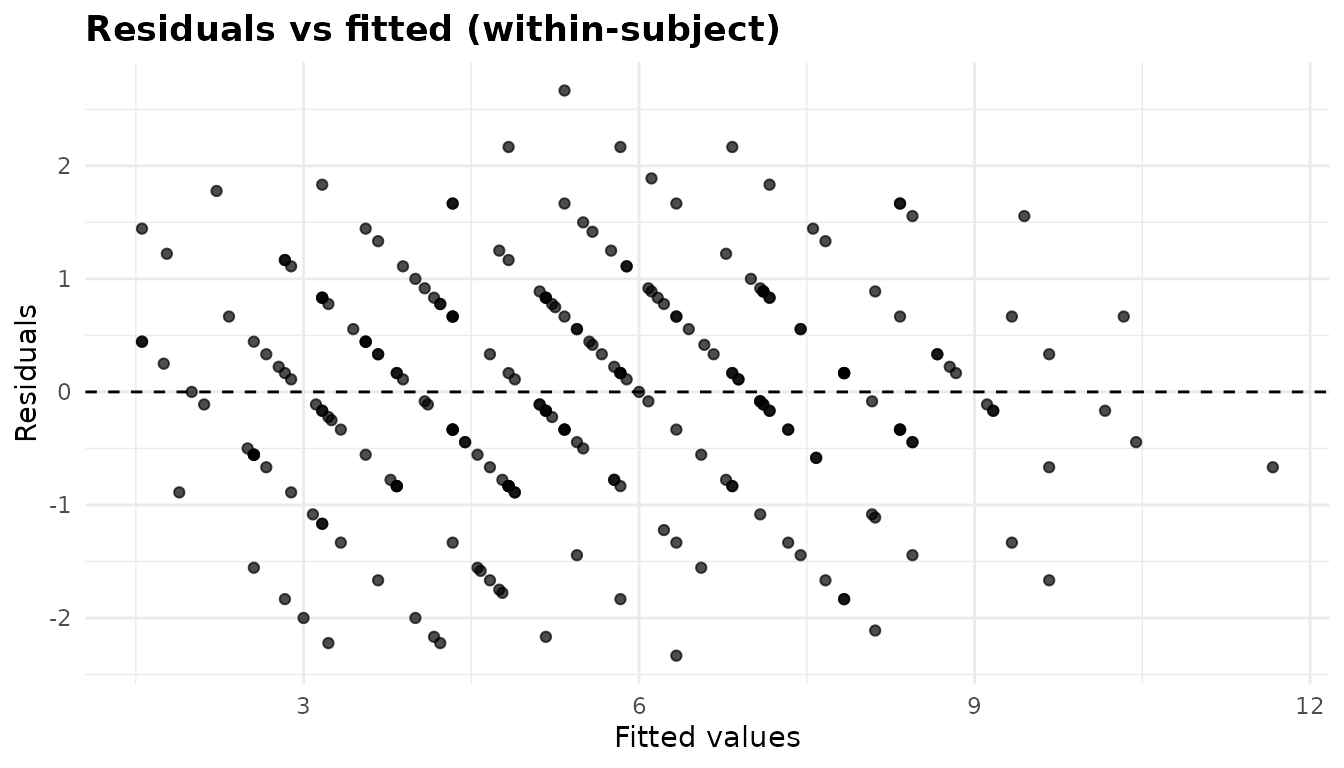

The residuals and fitted values are the within-subject ones described above (a fitted value is the observed value minus its residual). What to look for: the same even band as in any residual plot, with no funnel. The values in this data set are whole numbers on a short scale, which is why the points line up along diagonal stripes.

Normal Q-Q plot

plot(fit, "qq")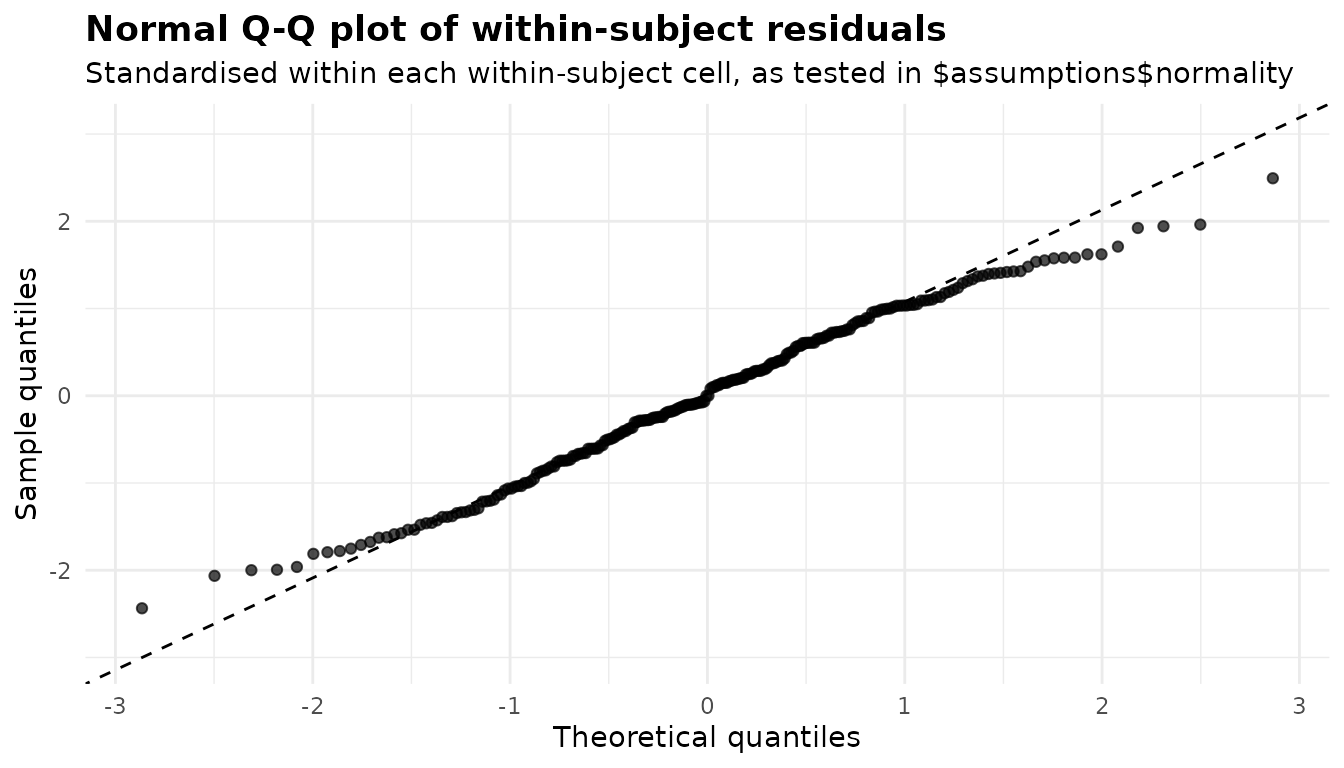

The residuals here are standardised within each within-subject cell, as they are tested in $assumptions$normality, so cells with different spreads are put on the same footing. What to look for: points along the dashed line, with no systematic curve at the ends. Here both ends bend in towards the middle: the residuals have lighter tails than a normal distribution, which is common for whole-number scores on a short scale and is generally harmless for the F tests. Heavy tails, bending away from the line, would be the worrying pattern.

Residuals in row order

plot(fit, "index")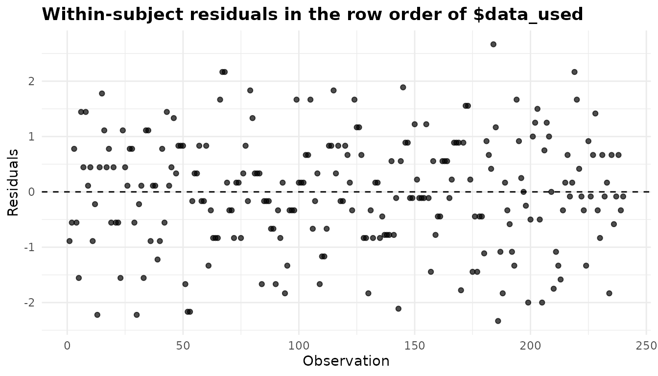

The residuals in the row order of $data_used, which is the order the rows came in (here, 15 consecutive rows per subject). What to look for: no trends, and no runs of residuals on the same side of zero. A drift within each block of rows would suggest practice or fatigue effects that the model does not capture; if your data are sorted by time of testing, this is where a drift over the course of the study would show. Nothing of the kind is visible here.

Marginal means

plot(fit, "emmeans")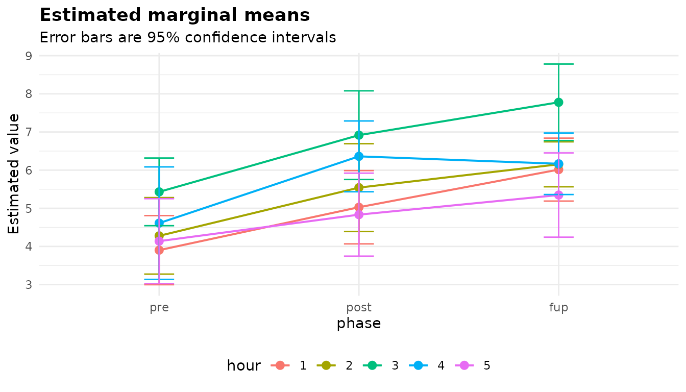

plot(tp, "emmeans")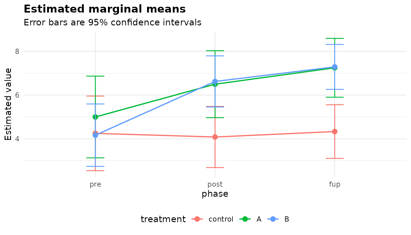

The first factor in emm_specs goes on the x axis and any others are mapped to colour, with one line per level. In the first plot (the default, phase by hour) the pre-test is the lowest phase at every hour and the third hour is the highest in every phase. The second, phase by treatment, shows the control group staying flat while A and B rise, which is the treatment:phase interaction.

Incomplete designs

A repeated measures ANOVA needs every subject in every within-subject cell. datasets::ChickWeight records the weights of 50 chicks on four diets, every two days from birth to day 20 and on day 21. Some chicks died or were not weighed on every day:

cw <- as.data.frame(datasets::ChickWeight)
table(table(cw$Chick))   # rows per chick: most have all 12
#> 
#>  2  7  8 10 11 12 
#>  1  1  1  1  1 45

Time is numeric; like every within-subject column it is turned into a factor, so each day is a level.

chick <- anova_rm(cw, "weight", subject = "Chick", within = "Time",
                  between = "Diet", plots = FALSE)
chick$subjects_dropped
#> [1] "18" "16" "15" "8"  "44"
c(n_removed = chick$n_removed,
  missing = chick$n_removed_missing,
  unbalanced = chick$n_removed_unbalanced,
  aggregated = chick$n_removed_aggregated)
#>  n_removed    missing unbalanced aggregated 
#>         38          0         38          0
chick$notes[1]
#> [1] "5 subject(s) were removed because they are missing at least one within-subject cell: 18, 16, 15, 8, 44. A repeated measures ANOVA requires a complete design."

Five chicks without a full set of weighings were removed before fitting, and they are listed in $subjects_dropped in the order of the subject column’s levels (Chick is an ordered factor, which is why they are not in numeric order). $n_removed counts every input row that is not in $data_used, and three components break it down by cause: rows with a missing value, rows belonging to incomplete subjects, and rows combined by aggregation (next section). Here all 38 removed rows belong to incomplete subjects.

A missing value costs more than its own row. Setting one weight to NA:

cw_na <- cw
cw_na$weight[cw_na$Chick == "1" & cw_na$Time == 10] <- NA
chick_na <- anova_rm(cw_na, "weight", subject = "Chick", within = "Time",
                     between = "Diet", plots = FALSE)
c(n_removed = chick_na$n_removed,
  missing = chick_na$n_removed_missing,
  unbalanced = chick_na$n_removed_unbalanced)
#>  n_removed    missing unbalanced 
#>         50          1         49
chick_na$subjects_dropped
#> [1] "18" "16" "15" "8"  "1"  "44"

The row with the missing weight is dropped, which leaves chick 1 without a day-10 weighing, so its other 11 rows go too. nrow(data_used) + n_removed is always the number of rows supplied. If losing whole subjects is too costly, a mixed model (for example with lme4 or afex’s mixed()) can use incomplete subjects; anova_rm() cannot.

These growth data also show how badly sphericity can fail: weights spread out as chicks grow, so the variance of the differences grows with the gap between days.

print(chick$sphericity[, c("term", "mauchly_w", "p_value", "gg_epsilon",
                           "hf_epsilon")], digits = 3)
#>        term mauchly_w   p_value gg_epsilon hf_epsilon
#> 1      Time  2.68e-17 1.03e-251      0.114      0.116
#> 2 Diet:Time  2.68e-17 1.03e-251      0.114      0.116

A Greenhouse-Geisser epsilon of 0.11 is close to its minimum of 1/11 for a 12-level factor: the corrected test has barely more degrees of freedom than a single comparison.

Internal names

afex builds a model formula from column names and names its wide-format columns after the within-subject levels, so a column called subject id or levels such as 0, 2, 4 would be mangled. anova_rm() therefore gives afex internal names and labels, and maps every table and plot back to yours. $model is the afex fit itself and keeps the internal names; $internal_names gives the correspondence:

chick$internal_names
#>       role   name internal
#> 1 response weight        Y
#> 2  subject  Chick       ID
#> 3   within   Time       W1
#> 4  between   Diet       B1
head(chick$model$data$long, 3)
#>    ID B1  W1  Y
#> 1 S01 L1 L01 41
#> 2 S01 L1 L02 48
#> 3 S01 L1 L03 53

The day levels 0, 2, 4, … are L01, L02, L03, … in $model, in level order. You only need this table if you work with $model directly.

Repeated rows: `fun_aggregate`

Sometimes a subject has several rows in the same cell: several trials per condition, or, if you leave a factor out of the analysis, the rows it used to distinguish. Analysing obk by phase alone leaves five rows (the hours) per subject and phase. They are combined into one value before fitting, with the mean by default:

by_phase <- anova_rm(obk, "value", subject = "id", within = "phase",
                     between = "treatment", plots = FALSE)
by_phase$notes[1]
#> [1] "48 subject-by-cell combination(s) have more than one row (192 extra row(s)); each was aggregated into one value with the mean (the default; pass fun_aggregate to choose another function) before fitting. $data_used holds the aggregated rows, and the 192 row(s) aggregated away are included in $n_removed."
c(used = nrow(by_phase$data_used), removed = by_phase$n_removed,
  aggregated = by_phase$n_removed_aggregated)
#>       used    removed aggregated 
#>         48        192        192
head(by_phase$data_used, 3)
#>   value id phase treatment
#> 1     2  1   pre   control
#> 2     3  1  post   control
#> 3     3  1   fup   control

$data_used holds the aggregated rows (one per subject and phase), and the 192 rows combined away are counted in $n_removed and $n_removed_aggregated. Pass fun_aggregate to use another function, for example the median for skewed trial-level data:

by_phase_md <- anova_rm(obk, "value", subject = "id", within = "phase",
                        between = "treatment", fun_aggregate = median,
                        plots = FALSE)
by_phase_md$notes[1]
#> [1] "48 subject-by-cell combination(s) have more than one row (192 extra row(s)); each was aggregated into one value with `median` before fitting. $data_used holds the aggregated rows, and the 192 row(s) aggregated away are included in $n_removed."
all.equal(by_phase_md$data_used$value, by_phase$data_used$value)
#> [1] TRUE

In these contrived data the median and the mean of each subject’s five hourly values happen to coincide, so the result is the same; the note records the function either way. Aggregation is a convenience: if the repeated rows are a design factor, like hour, it is usually better to keep it in within.

A within-only design

between is optional. datasets::sleep gives the extra hours of sleep of ten patients under two drugs (group), each patient taking both, so group is a within-subject factor and ID the subject:

sl <- anova_rm(datasets::sleep, "extra", subject = "ID", within = "group")
sl
#> Repeated measures analysis of variance 
#> --------------------------------------
#> Call: anova_rm(data = datasets::sleep, response = "extra", subject = "ID", within = "group")
#> Observations used: 20
#> 
#> Omnibus test (Type III, F, no sphericity correction)
#>    term num_df den_df    mse statistic partial_eta_sq  p_value
#> 1 group      1      9 0.7564      16.5         0.6471 0.002833
#> 
#> Notes
#>   - Sphericity is not an issue for this design: every within-subject factor has two levels, where the assumption holds automatically.
#> 
#> Plots available: residuals, qq, index, emmeans
#>   (use plot(x, which = "residuals"))

With a two-level factor there is only one difference per subject, so sphericity holds automatically: $sphericity is NULL and the note says why. The heading of the table says “no sphericity correction”, and attr(sl$anova, "correction") is “none”, even though correction was left at its default: there is nothing to correct, and the degrees of freedom are the uncorrected 1 and 9. The ANOVA is then the paired t-test in another form, with F = t²:

d <- with(datasets::sleep, extra[group == "2"] - extra[group == "1"])
tt <- t.test(d)
c(t_squared = unname(tt$statistic)^2, F = sl$anova$statistic,
  p_t = tt$p.value, p_F = sl$anova$p_value)
#>   t_squared           F         p_t         p_F 
#> 16.50088132 16.50088132  0.00283289  0.00283289

The same equivalence holds for the normality check. With one two-level within-subject factor, the residuals are plus and minus half of each subject’s centred difference, so both rows of $assumptions$normality test the normality of the differences, which is exactly the assumption of the paired t-test:

sl$assumptions$normality
#>   cell  n statistic    p_value note
#> 1    1 10 0.8298713 0.03334161 <NA>
#> 2    2 10 0.8298713 0.03334161 <NA>
shapiro.test(d)$p.value
#> [1] 0.03334161

Both rows give p = 0.033: the differences are not convincingly normal, because one patient’s difference (4.6 hours) is far larger than the others (without that patient, Shapiro-Wilk gives p = 0.77). Ten subjects is too few to lean on the test, but it is a reason to check the result with a nonparametric paired test.

Options worth knowing

correction ("GG", "HF", "none"), shown above.
emm_specs, shown above. When it leaves out a factor of the model, the means are averaged over it and a note says so.
adjust sets the multiplicity adjustment for $posthoc: "tukey" (the default), "holm", "bonferroni", "BH" and others; posthoc = FALSE skips the comparisons.
conf_level sets the level of every interval.
A few arguments of afex::aov_ez() pass through ...: observed (above), fun_aggregate (above), type = 2 for Type II sums of squares, and anova_table = list(p_adjust_method = "holm") to adjust the p-values of $anova across its terms. Anything else is an error rather than silently ignored. covariate is refused: anova_rm() does not fit covariates.

t2 <- anova_rm(obk, "value", subject = "id", within = c("phase", "hour"),
               between = c("treatment", "gender"), type = 2, plots = FALSE)
attr(t2$anova, "ss_type")
#> [1] "II"
print(t2$anova[1:3, c("term", "statistic", "p_value")], digits = 3)
#>               term statistic p_value
#> 1        treatment      4.63  0.0377
#> 2           gender      2.56  0.1410
#> 3 treatment:gender      2.86  0.1045

The design here is unbalanced between subjects (two to four subjects per treatment-by-gender cell), so Type II and Type III tests differ for most terms. Only the terms that contain both between-subject factors, such as treatment:gender, are the same under both.

factorize = TRUE (the default) converts a response stored as a factor or as text to numbers through its labels, so a factor with levels 11, 17, 21 becomes 11, 17, 21 rather than 1, 2, 3; a note records the conversion.

What the notes say

fit$notes
#> [1] "Mauchly's test rejects sphericity for hour, treatment:hour, gender:hour, treatment:gender:hour; the reported table uses the Greenhouse-Geisser correction."                                                                                                                                                                                                                                    
#> [2] "The marginal means in $emmeans and the comparisons in $posthoc are averaged over the levels of: treatment, gender. The ANOVA table shows a significant interaction with a factor averaged over (treatment:phase, p = 0.0127), so these averages can hide or reverse the differences within its levels; set emm_specs = c(\"phase\", \"hour\", \"treatment\", \"gender\") to compare the cells."

Mauchly’s test rejects sphericity for hour and the terms involving it, and the table uses the Greenhouse-Geisser correction. The corrected p-values are the ones to report.
The default marginal means average over treatment and gender, but treatment:phase is significant, so those averages can hide the difference between treatments. The note suggests the full cell grid; a smaller emm_specs such as c("phase", "treatment"), used above, is often enough.

Other notes you may see: subjects removed for incomplete cells, rows aggregated, a response converted from a factor, epsilons computed directly because the error matrix is singular, a Huynh-Feldt estimate above 1, a design with no error degrees of freedom, and anything afex or emmeans said while the model was being fitted.

Reporting the result

A 3 (treatment) x 2 (gender) x 3 (phase) x 5 (hour) mixed ANOVA was run on the scores, with Type III sums of squares and Greenhouse-Geisser corrected degrees of freedom (Mauchly’s test rejected sphericity for hour, W = 0.07, p = 0.0076; epsilon = 0.46). Scores changed across phases, F(1.60, 15.99) = 16.13, p < 0.001, generalised η² = 0.22, and across hours, F(1.84, 18.41) = 16.69, p < 0.001, generalised η² = 0.18. The change across phases depended on treatment, F(3.20, 15.99) = 4.85, p = 0.013, generalised η² = 0.14: averaged over hour and gender, the control group scored 4.25 at pre-test and 4.33 at follow-up, against 5.00 to 7.25 for treatment A and 4.17 to 7.29 for treatment B.