MANOVA: comparing groups on several responses at once

library(anovakit)

anova_manova() compares two or more numeric responses jointly across groups. It reports a multivariate test of each term, follows it up with one ANOVA per response, and describes how the groups separate with a canonical discriminant analysis; with covariates it becomes a MANCOVA. Use it when you have several related measurements on each unit and want one test of “do the groups differ on these measurements taken together”, or want to know which combination of them separates the groups. For a single response use anova_glm(), anova_welch() or, with a covariate, anova_ancova(); for the same response measured repeatedly on each subject, anova_rm(). The decision guide has more.

The data

datasets::iris gives four measurements, in centimetres, of 50 flowers from each of three species of iris.

resp <- c("Sepal.Length", "Sepal.Width", "Petal.Length", "Petal.Width")
head(iris)
#>   Sepal.Length Sepal.Width Petal.Length Petal.Width Species
#> 1          5.1         3.5          1.4         0.2  setosa
#> 2          4.9         3.0          1.4         0.2  setosa
#> 3          4.7         3.2          1.3         0.2  setosa
#> 4          4.6         3.1          1.5         0.2  setosa
#> 5          5.0         3.6          1.4         0.2  setosa
#> 6          5.4         3.9          1.7         0.4  setosa
table(iris$Species)
#> 
#>     setosa versicolor  virginica 
#>         50         50         50
aggregate(. ~ Species, data = iris, FUN = mean)
#>      Species Sepal.Length Sepal.Width Petal.Length Petal.Width
#> 1     setosa        5.006       3.428        1.462       0.246
#> 2 versicolor        5.936       2.770        4.260       1.326
#> 3  virginica        6.588       2.974        5.552       2.026

The four measurements are strongly correlated with each other (bigger flowers are bigger in every direction), so four separate ANOVAs would test largely the same thing four times. A MANOVA tests them together, taking the correlations into account.

Fitting the model

Responses are named as a character vector, then the grouping variable(s).

fit <- anova_manova(iris, resp, "Species")
fit
#> Multivariate analysis of variance (Pillai test, Type II) 
#> --------------------------------------------------------
#> Call: anova_manova(data = iris, responses = resp, groups = "Species")
#> Observations used: 150
#> 
#> Omnibus test (Type II, Pillai's trace, approximate F)
#>      term df statistic approx_f num_df den_df   p_value
#> 1 Species  2     1.192    53.47      8    290 < 2.2e-16
#> 
#> Notes
#>   - Mardia's tests reject multivariate normality of the residuals. The multivariate table uses Pillai's trace, the most robust of the four statistics to this.
#>   - Box's M rejects equality of the group covariance matrices. The test is very sensitive to non-normality, so inspect the group covariances before acting on it. With equal group sizes the multivariate tests are fairly robust to unequal covariances, Pillai's trace most of all (it is the statistic used here).
#> 
#> Plots available: residuals_Sepal.Length, qq_Sepal.Length, residuals_Sepal.Width, qq_Sepal.Width, residuals_Petal.Length, qq_Petal.Length, residuals_Petal.Width, qq_Petal.Width, emmeans, canonical
#>   (use plot(x, which = "residuals_Sepal.Length"))

Reading the printout:

The method line names the multivariate statistic (Pillai’s trace, the default test) and the type of test (Type II, the default type).
Observations used: 150: no rows were dropped.
The table is the multivariate test, one row per term.
The notes say that Mardia’s tests reject multivariate normality and that Box’s M rejects equal covariance matrices. Both are discussed below.
There are two plots per response (residuals and Q-Q), a marginal-means plot and a canonical plot.

summary(fit) adds the assumption checks, the effect sizes, marginal means and comparisons for every response, the canonical axes and each response’s univariate ANOVA table.

The multivariate test

fit$multivariate
#>      term df statistic approx_f num_df den_df      p_value
#> 1 Species  2  1.191899 53.46649      8    290 9.742163e-53
attr(fit$multivariate, "statistic")
#> [1] "Pillai's trace, approximate F"

$multivariate (the same table as $anova) has one row per term:

df is the term’s hypothesis degrees of freedom (a three-level factor has 2).
statistic is the multivariate statistic, here Pillai’s trace, which lies between 0 and the smaller of the number of responses and df.
approx_f, num_df and den_df are its F approximation, and p_value the p-value from it.

The tests are computed by car::Manova() on the multivariate linear model lm(cbind(<responses>) ~ <groups>), kept in $model. They are Type II by default: each term is adjusted for every other term that does not contain it, so the result does not depend on the order of groups. type = "III" fits under sum-to-zero contrasts and adjusts each term for all others. With one grouping variable the two agree, and both agree with summary(stats::manova()), which is sequential and so order-dependent once there are several terms.

Here the species differ overwhelmingly on the four measurements taken together (Pillai’s trace = 1.192, p far below any threshold).

Which statistic: `test`

There are four standard multivariate statistics, and test chooses one: "Pillai" (the default), "Wilks", "Hotelling-Lawley" or "Roy". They are all functions of the same eigenvalues and usually agree, as here:

tests <- c("Pillai", "Wilks", "Hotelling-Lawley", "Roy")
do.call(rbind, lapply(tests, function(t) {
  f <- anova_manova(iris, resp, "Species", test = t, plots = FALSE)
  data.frame(test = t, f$multivariate[, c("statistic", "approx_f", "num_df",
                                          "den_df", "p_value")])
}))
#>               test   statistic   approx_f num_df den_df       p_value
#> 1           Pillai  1.19189883   53.46649      8    290  9.742163e-53
#> 2            Wilks  0.02343863  199.14534      8    288 1.365006e-112
#> 3 Hotelling-Lawley 32.47732024  580.53210      8    286 6.436176e-172
#> 4              Roy 32.19192920 1166.95743      4    145 3.787298e-109

They differ in how they behave when the assumptions fail and in which alternatives they detect best. Pillai’s trace is the most robust to unequal covariance matrices and non-normality, which is why it is the default. Roy’s largest root uses only the first eigenvalue: it is the most powerful when the groups differ along a single direction, but with more than one hypothesis degree of freedom its F statistic is only an upper bound, so its p-value is a lower bound, and a note says so:

roy <- anova_manova(iris, resp, "Species", test = "Roy", plots = FALSE)
roy$notes
#> [1] "For `Species`, Roy's largest root has only an upper bound for its F statistic (the hypothesis has more than one degree of freedom and there are 4 responses), so the reported p-value is a lower bound: it is anti-conservative. Pillai's trace or Wilks' lambda give calibrated p-values."                    
#> [2] "Mardia's tests reject multivariate normality of the residuals. Pillai's trace is the most robust of the four multivariate statistics to this; consider test = \"Pillai\"."                                                                                                                                     
#> [3] "Box's M rejects equality of the group covariance matrices. The test is very sensitive to non-normality, so inspect the group covariances before acting on it. With equal group sizes the multivariate tests are fairly robust to unequal covariances, Pillai's trace most of all (consider test = \"Pillai\")."
roy$test
#> [1] "Roy"

Univariate follow-ups

A significant multivariate test says the groups differ somewhere in the four measurements. The follow-ups say where. One ANOVA (of the same type as the multivariate test) is fitted per response and kept under $univariate, each with its own model, table, effect sizes, marginal means, emmeans grid and comparisons:

names(fit$univariate)
#> [1] "Sepal.Length" "Sepal.Width"  "Petal.Length" "Petal.Width"
names(fit$univariate$Sepal.Width)
#> [1] "model"          "anova"          "effect_sizes"   "emmeans"       
#> [5] "emmeans_object" "posthoc"
fit$univariate$Sepal.Width$anova
#>        term   sum_sq  df statistic      p_value
#> 1   Species 11.34493   2  49.16004 4.492017e-17
#> 2 Residuals 16.96200 147        NA           NA

The univariate p-values are not adjusted across responses, and they are reported whether or not the multivariate test is significant. When a term’s multivariate test is not significant at the 0.05 level, a note says that its follow-ups are not protected by it. Treat a small univariate p-value there as a lead, not a finding.

Effect sizes

$effect_sizes stacks the partial eta squared and partial omega squared of every term in every response’s ANOVA, with a response column:

fit$effect_sizes
#>       response    term df    sum_sq partial_eta_sq partial_omega_sq
#> 1 Sepal.Length Species  2  63.21213      0.6187057        0.6119308
#> 2  Sepal.Width Species  2  11.34493      0.4007828        0.3910362
#> 3 Petal.Length Species  2 437.10280      0.9413717        0.9401991
#> 4  Petal.Width Species  2  80.41333      0.9288829        0.9274667

Species accounts for 94% of the variation in petal length but only 40% of the variation in sepal width. No multivariate effect size is reported; a common one is Pillai’s trace divided by the smaller of the number of responses and df, here 1.192 / 2 = 0.60.

Marginal means and comparisons

The marginal means and comparisons of every response are stacked in one table each, with a response column:

print(fit$emmeans, digits = 3)
#>        response    Species estimate     se  df conf_low conf_high
#> 1  Sepal.Length     setosa    5.006 0.0728 147    4.862     5.150
#> 2  Sepal.Length versicolor    5.936 0.0728 147    5.792     6.080
#> 3  Sepal.Length  virginica    6.588 0.0728 147    6.444     6.732
#> 4   Sepal.Width     setosa    3.428 0.0480 147    3.333     3.523
#> 5   Sepal.Width versicolor    2.770 0.0480 147    2.675     2.865
#> 6   Sepal.Width  virginica    2.974 0.0480 147    2.879     3.069
#> 7  Petal.Length     setosa    1.462 0.0609 147    1.342     1.582
#> 8  Petal.Length versicolor    4.260 0.0609 147    4.140     4.380
#> 9  Petal.Length  virginica    5.552 0.0609 147    5.432     5.672
#> 10  Petal.Width     setosa    0.246 0.0289 147    0.189     0.303
#> 11  Petal.Width versicolor    1.326 0.0289 147    1.269     1.383
#> 12  Petal.Width  virginica    2.026 0.0289 147    1.969     2.083

print(fit$posthoc[, c("response", "contrast", "estimate", "conf_low",
                      "conf_high", "p_value", "p_adjusted")], digits = 3)
#>        response               contrast estimate conf_low conf_high  p_value
#> 1  Sepal.Length    setosa - versicolor   -0.930   -1.174   -0.6862 8.77e-16
#> 2  Sepal.Length     setosa - virginica   -1.582   -1.826   -1.3382 2.21e-32
#> 3  Sepal.Length versicolor - virginica   -0.652   -0.896   -0.4082 2.77e-09
#> 4   Sepal.Width    setosa - versicolor    0.658    0.497    0.8189 1.83e-17
#> 5   Sepal.Width     setosa - virginica    0.454    0.293    0.6149 4.54e-10
#> 6   Sepal.Width versicolor - virginica   -0.204   -0.365   -0.0431 3.15e-03
#> 7  Petal.Length    setosa - versicolor   -2.798   -3.002   -2.5942 5.25e-69
#> 8  Petal.Length     setosa - virginica   -4.090   -4.294   -3.8862 4.11e-91
#> 9  Petal.Length versicolor - virginica   -1.292   -1.496   -1.0882 1.81e-31
#> 10  Petal.Width    setosa - versicolor   -1.080   -1.177   -0.9831 1.25e-57
#> 11  Petal.Width     setosa - virginica   -1.780   -1.877   -1.6831 7.95e-86
#> 12  Petal.Width versicolor - virginica   -0.700   -0.797   -0.6031 8.82e-37
#>    p_adjusted
#> 1    3.39e-14
#> 2    3.00e-15
#> 3    8.29e-09
#> 4    3.10e-14
#> 5    1.36e-09
#> 6    8.78e-03
#> 7    3.00e-15
#> 8    3.00e-15
#> 9    3.00e-15
#> 10   3.00e-15
#> 11   3.00e-15
#> 12   3.00e-15

p_value is unadjusted and p_adjusted is adjusted by the method in the adjustment column (Tukey by default). The adjust argument controls the adjustment within each response only: here each response’s three comparisons are one family, and nothing is adjusted across the four responses. If you report comparisons for all responses, say so, or adjust the p_value column across the whole table yourself with p.adjust(). The many identical p_adjusted values of about 3e-15 are not a coincidence: Tukey p-values come from ptukey(), whose upper tail has an absolute error of about 1e-14, so digits below about 1e-10 are noise, and summary(fit) prints such values as < 1e-10.

Without covariates the marginal means are the raw group means, since there is nothing to adjust for. $emmeans_object is NULL because there is one emmeans grid per response; take the one you need from $univariate:

is.null(fit$emmeans_object)
#> [1] TRUE
class(fit$univariate$Petal.Width$emmeans_object)
#> [1] "emmGrid"
#> attr(,"package")
#> [1] "emmeans"

Canonical discriminant analysis

The multivariate test says the species differ; the canonical discriminant analysis says how. It finds the weighted combinations of the responses (the canonical axes) that separate the groups best relative to the variation within groups:

fit$canonical
#>   axis eigenvalue canonical_r prop_variance
#> 1 Can1  32.191929   0.9848209   0.991212605
#> 2 Can2   0.285391   0.4711970   0.008787395
fit$canonical_term
#> [1] "Species"

eigenvalue is the ratio of between-group to within-group variation along the axis.
canonical_r is the correlation between the axis and the group membership.
prop_variance is the axis’s share of the term’s between-group variation.

There are at most min(number of responses, df) axes, here two. The first carries 99.1% of the separation: the three species lie almost along a single line. To see what the axes mean, read the structure coefficients, the pooled within-group correlations between each response and each axis:

fit$assumptions$structure_coefficients
#>       response       Can1      Can2
#> 1 Sepal.Length  0.2225959 0.3108117
#> 2  Sepal.Width -0.1190115 0.8636809
#> 3 Petal.Length  0.7060654 0.1677014
#> 4  Petal.Width  0.6331779 0.7372421

Can1 is mainly petal length and petal width; Can2 is mainly sepal width, with petal width. The sign of an axis is arbitrary; the function makes each axis’s largest structure coefficient positive so the orientation is reproducible.

$canonical_term names the term the analysis describes, spelled as in $multivariate$term. With one grouping variable that is the grouping term. With several, it is their full interaction when the model contains it, and otherwise the first grouping variable; see below.

Checking assumptions

MANOVA assumes that the residuals are multivariate normal and that every group has the same covariance matrix. Iris is the textbook example where the second assumption fails.

names(fit$assumptions)
#> [1] "mardia"                 "box_m"                  "cell_counts"           
#> [4] "structure_coefficients"
fit$assumptions$mardia
#>              test statistic df     p_value
#> 1 Mardia skewness 31.848063 20 0.044944433
#> 2 Mardia kurtosis  3.281965 NA 0.001030865
fit$assumptions$box_m
#>   statistic df      p_value
#> 1   140.943 20 3.352034e-20
fit$assumptions$cell_counts
#>         cell  n
#> 1     setosa 50
#> 2 versicolor 50
#> 3  virginica 50

mardia holds Mardia’s tests of multivariate skewness and kurtosis, on the residuals of the multivariate model. Both reject here (skewness p = 0.045, kurtosis p = 0.001). They are asymptotic, and the kurtosis test rejects too often when the sample is small relative to the square of the number of responses. The tests are skipped, with a note, unless the residual degrees of freedom exceed the number of responses by at least 10.
box_m is Box’s M test of equal covariance matrices across the cells of the grouping variables. It rejects decisively (statistic 140.9 on 20 df).
cell_counts gives the number of observations in each cell.
structure_coefficients belongs to the canonical analysis above.

The variances of each measurement within each species show what Box’s M is reacting to:

vars <- sapply(split(iris[resp], iris$Species), function(d) diag(var(d)))
round(vars, 3)
#>              setosa versicolor virginica
#> Sepal.Length  0.124      0.266     0.404
#> Sepal.Width   0.144      0.098     0.104
#> Petal.Length  0.030      0.221     0.305
#> Petal.Width   0.011      0.039     0.075

Setosa’s petals vary far less than the other two species’: the variance of its petal length is 0.030 cm², against 0.221 and 0.305. So what should you do? Box’s M is notoriously sensitive to non-normality, and it will reject for differences that do not matter in large samples, so treat it as a prompt to look at the group covariances, as above, rather than as a verdict. What matters for the multivariate test is how the covariance difference combines with the group sizes. With equal group sizes, as here, Pillai’s trace is robust to unequal covariance matrices; with unequal sizes and unequal covariances, the test is liberal when the smaller groups have the larger covariances, and Pillai’s trace is still the safest choice. The Box’s M note makes the same distinction: it checks whether the group sizes are equal and says whether Pillai’s trace is the statistic in use (see What the notes say). With a separation this strong, no reasonable violation would change the conclusion.

The diagnostics article covers the checks across the package. The checks cost time on a large data set; assumptions = FALSE skips Mardia’s tests and Box’s M, leaving only the cell counts and the structure coefficients:

quick <- anova_manova(iris, resp, "Species", assumptions = FALSE,
                      plots = FALSE)
names(quick$assumptions)
#> [1] "cell_counts"            "structure_coefficients"
quick$notes
#> character(0)

Plots

Each plot is a ggplot2 object in $plots, returned by plot(fit, "name") and modifiable with + (see Plots and visual customisation).

names(fit$plots)
#>  [1] "residuals_Sepal.Length" "qq_Sepal.Length"        "residuals_Sepal.Width" 
#>  [4] "qq_Sepal.Width"         "residuals_Petal.Length" "qq_Petal.Length"       
#>  [7] "residuals_Petal.Width"  "qq_Petal.Width"         "emmeans"               
#> [10] "canonical"

Residuals and Q-Q plots, per response

Each response’s univariate model has its own residuals-against-fitted plot, residuals_<response>, and normal Q-Q plot, qq_<response>. The two for petal length:

plot(fit, "residuals_Petal.Length")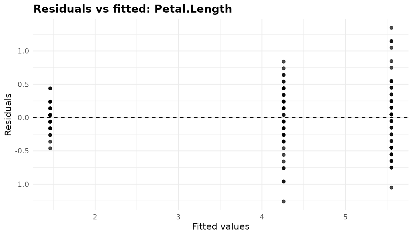

The fitted values of a one-way model are the group means, so the points fall in three vertical strips, one per species. What to look for: similar spread in each strip. Here the setosa strip (fitted value near 1.5 cm) is far narrower than the other two, the unequal variances seen above.

plot(fit, "qq_Petal.Length")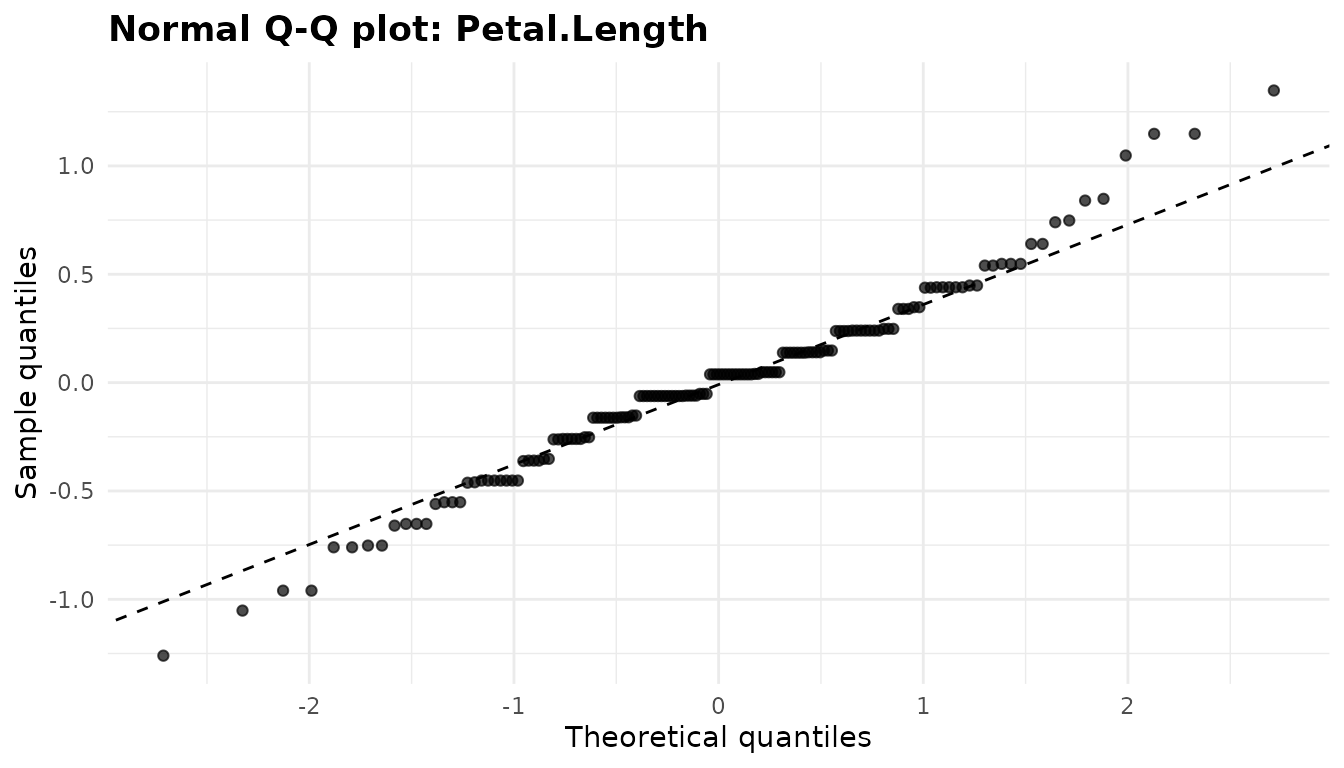

What to look for: points along the dashed line. These residuals follow it closely in the middle, and both tails are a little longer than a normal distribution’s (points above the line at the top, below it at the bottom). The residuals_Sepal.Length, qq_Sepal.Length and so on are read the same way.

Marginal means

plot(fit, "emmeans")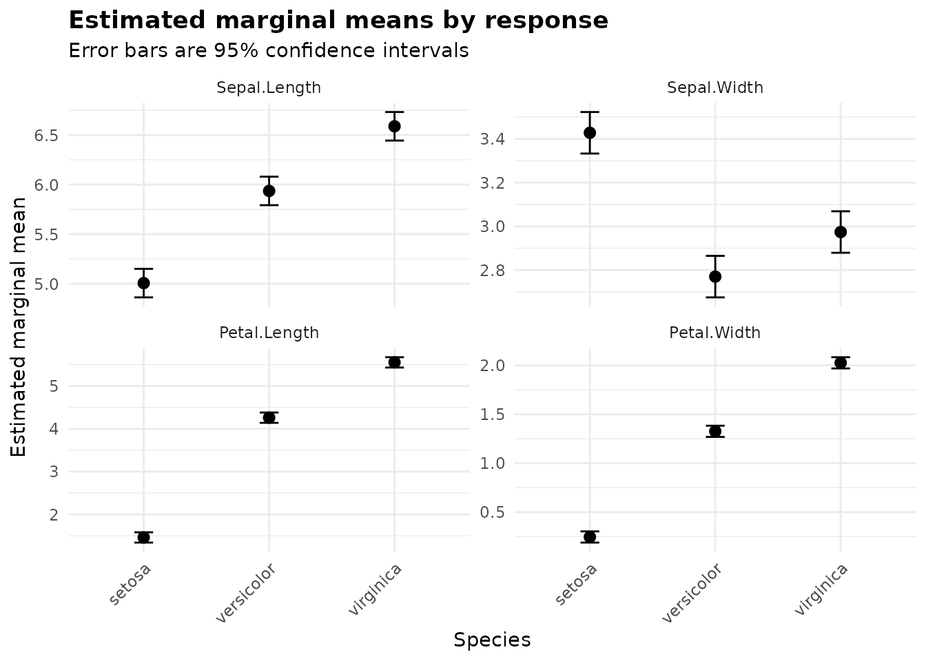

One panel per response, each on its own scale, with the marginal means and their confidence intervals. The panels show at a glance that setosa is the odd one out, and that sepal width is the only measurement on which it is the largest.

Canonical plot

plot(fit, "canonical")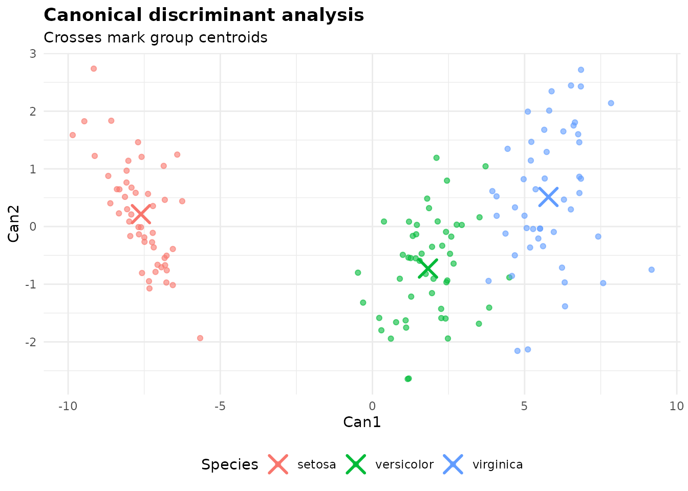

Every flower’s scores on the first two canonical axes, with crosses at the species centroids. The axes are scaled to unit pooled within-group variance, so the distance between centroids is in within-group standard deviations. What to look for: how far apart the groups are along each axis. Here the species are spread along Can1 with setosa well clear of the other two, while Can2 separates them far less, as its eigenvalue says. With only one estimable axis the plot becomes a box plot of Can1 by group, subtitled “Only one discriminant axis is estimable”, as in the examples below.

MANCOVA: adding covariates

covariates turns the analysis into a MANCOVA. MASS::survey records the span of the writing hand (Wr.Hnd) and the other hand (NW.Hnd), in centimetres, and the height of 237 students. Men have larger hands, but they are also taller; adjusting for height asks whether the hands differ between men and women of the same height.

sv <- MASS::survey
mc <- anova_manova(sv, c("Wr.Hnd", "NW.Hnd"), "Sex", covariates = "Height")
mc$multivariate
#>     term df statistic approx_f num_df den_df      p_value
#> 1 Height  1 0.1108827 12.65816      2    203 6.596988e-06
#> 2    Sex  1 0.1540809 18.48784      2    203 4.206061e-08
mc$n_removed
#> [1] 30

30 rows with a missing value in one of the four columns were dropped (the notes say which columns). The multivariate table now has a row for the covariate as well as for Sex.

Centring and adjusted means

Covariates are mean-centred before fitting. Centring changes no test here; it keeps a covariate with a large offset and a small spread from being mistaken for a constant, and it means the adjusted means are read at the covariate means, which are kept in $covariate_means:

mc$covariate_means
#>   Height 
#> 172.3845
print(mc$emmeans, digits = 4)
#>   response    Sex estimate     se  df conf_low conf_high
#> 1   Wr.Hnd Female    18.01 0.1684 204    17.68     18.34
#> 2   Wr.Hnd   Male    19.45 0.1652 204    19.13     19.78
#> 3   NW.Hnd Female    17.82 0.1753 204    17.47     18.16
#> 4   NW.Hnd   Male    19.50 0.1721 204    19.16     19.84
aggregate(cbind(Wr.Hnd, NW.Hnd) ~ Sex, data = mc$data_used, FUN = mean)
#>      Sex   Wr.Hnd   NW.Hnd
#> 1 Female 17.56078 17.41275
#> 2   Male 19.89048 19.89333

The raw difference in writing-hand span between the sexes, on these same rows, is 2.33 cm; at the mean height of 172.4 cm it is 1.45 cm. About 38% of the raw difference goes with height, and a clear difference remains.

Homogeneity of regression slopes

A MANCOVA assumes each covariate has the same slope in every group. The function tests this by comparing the model with one in which the covariate interacts with every grouping term, using the chosen multivariate statistic:

mc$slopes_test
#>                                   comparison df   statistic  approx_f num_df
#> 1 common slopes vs covariate-by-group slopes  1 0.004582515 0.4649647      2
#>   den_df   p_value homogeneous
#> 1    202 0.6288279        TRUE

The slopes are consistent with being equal here (p = 0.63). When the test rejects at the 0.05 level a note says so: the common-slope adjusted means then describe the groups at the covariate mean only, and the advice is to model the interaction yourself or analyse each response with anova_ancova(), which chooses between the two models and reports per-group slopes.

With covariates, the assumption checks and the canonical analysis work in the space the multivariate test operates in: Mardia’s tests use the residuals of the multivariate model, Box’s M compares the covariance matrices of the responses with the covariate effects removed, and the canonical scores have the covariate effects removed. A note records this:

mc$notes
#> [1] "Dropped 30 row(s) with missing values in: Wr.Hnd, NW.Hnd, Sex, Height."                                                                                                                                                             
#> [2] "Covariate(s) mean-centred before fitting (Height: 172.385), so $emmeans are adjusted means at the covariate mean(s). Centring changes no test."                                                                                     
#> [3] "Box's M compares the cell covariance matrices of the responses with the covariate effects removed (as estimated in the full model), and Mardia's tests use the model residuals: the conditional distribution the MANCOVA assumes."  
#> [4] "Mardia's tests reject multivariate normality of the residuals. The multivariate table uses Pillai's trace, the most robust of the four statistics to this."                                                                         
#> [5] "The canonical discriminant analysis describes the `Sex` term only: it is the grouping term. The model has 2 terms (Height, Sex); the canonical scores have the fitted effects of the other terms removed, so they show `Sex` alone."

Sex has one degree of freedom, so there is one canonical axis, and the canonical plot shows it as a box plot by group, subtitled “Only one discriminant axis is estimable”. Because the model has two terms, the subtitle also names the term the axis describes and says that the other terms’ effects (here, height’s) were removed:

plot(mc, "canonical")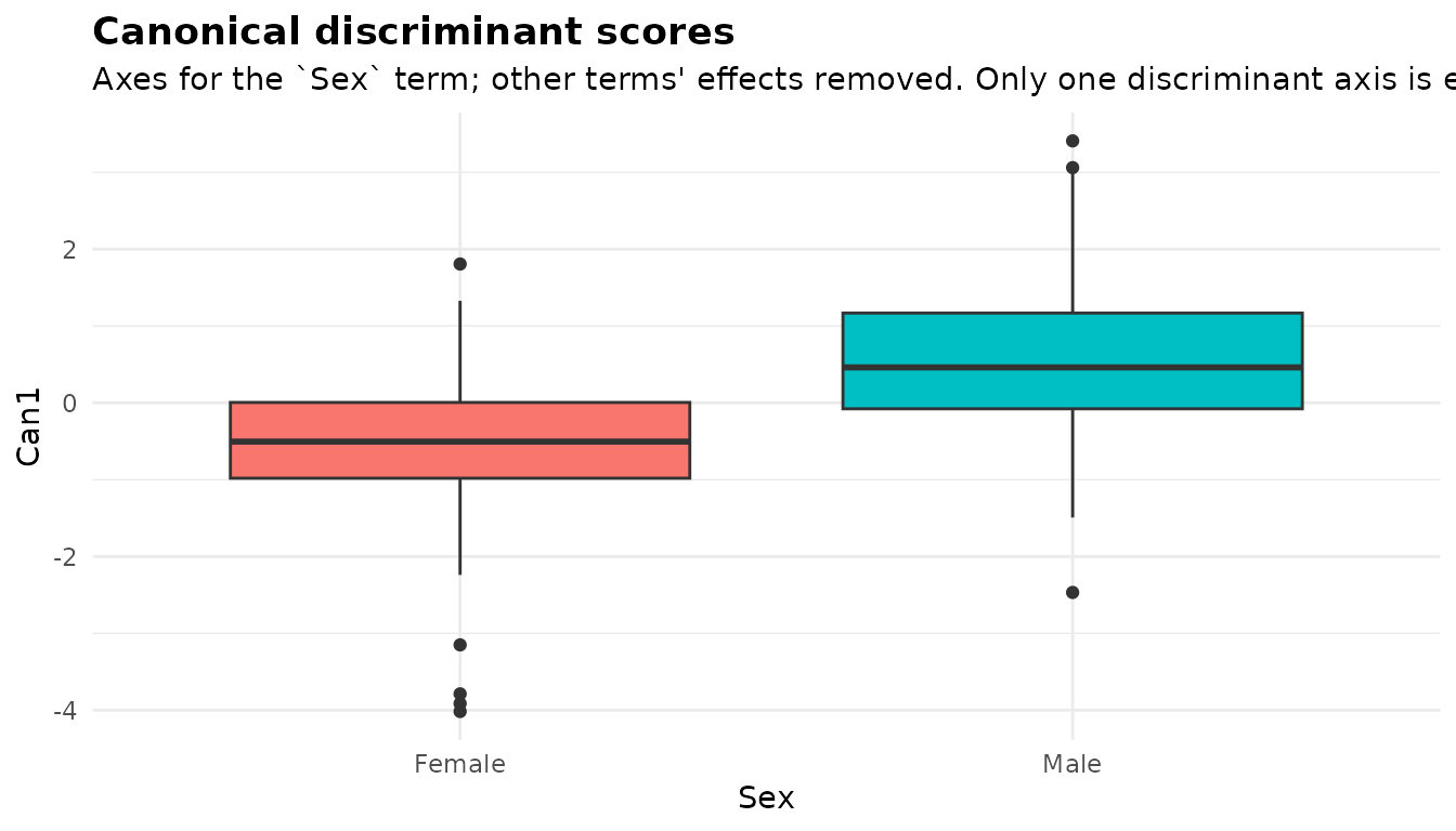

Men score higher on the axis, but the boxes overlap: at the same height, hand span separates the sexes only partly (canonical r = 0.39).

Several grouping variables

MASS::crabs has five body measurements (in millimetres) of 200 crabs, 50 of each sex (sex) in each of two colour forms (sp, blue or orange).

crabs <- MASS::crabs
crab_resp <- c("FL", "RW", "CL", "CW", "BD")
cr <- anova_manova(crabs, crab_resp, c("sp", "sex"), interaction = TRUE)
cr$multivariate
#>     term df statistic  approx_f num_df den_df      p_value
#> 1     sp  1 0.8796085 280.55931      5    192 3.256551e-86
#> 2    sex  1 0.7702723 128.75442      5    192 2.326195e-59
#> 3 sp:sex  1 0.2284959  11.37291      5    192 1.268967e-09
cr$assumptions$cell_counts
#>    cell  n
#> 1 B : F 50
#> 2 O : F 50
#> 3 B : M 50
#> 4 O : M 50

interaction is FALSE by default in anova_manova(), so the grouping variables enter additively unless you ask; TRUE fits the full factorial and a whole number keeps interactions up to that order. Here the colour-by-sex interaction is clear: the difference between the sexes in these measurements is not the same in the two colour forms.

With the full factorial, $emmeans and $posthoc compare the cells, and the marginal-means plot puts the first grouping variable on the x axis with one line per level of the others:

plot(cr, "emmeans")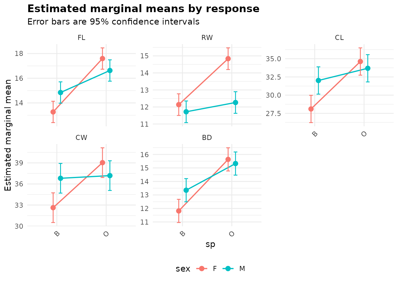

The canonical analysis describes a single term, which $canonical_term names. With the full interaction in the model it is that interaction, and the scores have the fitted effects of the main effects removed, so the plot shows the interaction alone:

cr$canonical_term
#> [1] "sp:sex"
cr$canonical
#>   axis eigenvalue canonical_r prop_variance
#> 1 Can1  0.2961694   0.4780125             1
plot(cr, "canonical")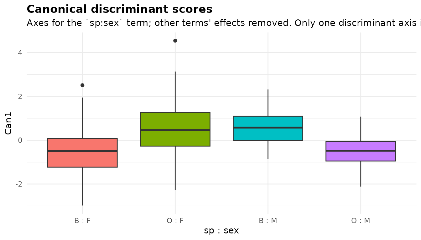

sp:sex has one degree of freedom, so there is one axis, and the subtitle says so. With the main effects removed, the scores show the interaction contrast itself: blue females and orange males on one side, orange females and blue males on the other. Without the interaction, the analysis describes the main effect of the first grouping variable; list another variable first in groups to describe it instead. In an additive model, $emmeans and $posthoc are reported for each factor separately, averaged over the others, with a term column:

cr_add <- anova_manova(crabs, crab_resp, c("sex", "sp"), plots = FALSE)
cr_add$canonical_term
#> [1] "sex"
head(cr_add$emmeans[, c("response", "term", "sex", "sp", "estimate")], 4)
#>   response term  sex   sp estimate
#> 1       FL  sex    F <NA>   15.432
#> 2       FL  sex    M <NA>   15.734
#> 3       FL   sp <NA>    B   14.056
#> 4       FL   sp <NA>    O   17.110

Options worth knowing

test chooses the multivariate statistic (above).
type = "III" gives Type III tests, for the multivariate table and the univariate follow-ups alike. If the model has aliased coefficients (an empty cell, collinear covariates), Type III is not defined, and Type II is used with a note.
interaction chooses how several grouping variables combine (above).
adjust sets the adjustment of the comparisons within each response (default "tukey"); posthoc = FALSE skips them.
conf_level sets the level of every interval.
assumptions = FALSE skips Mardia’s tests and Box’s M (above); the slopes test is always computed when there are covariates.
plots = FALSE skips building the plots, which saves time: there are two per response.
A single response is accepted, and falls back to a univariate analysis with a note; there is then no multivariate test and no canonical analysis.

What the notes say

fit$notes
#> [1] "Mardia's tests reject multivariate normality of the residuals. The multivariate table uses Pillai's trace, the most robust of the four statistics to this."                                                                                                                                                       
#> [2] "Box's M rejects equality of the group covariance matrices. The test is very sensitive to non-normality, so inspect the group covariances before acting on it. With equal group sizes the multivariate tests are fairly robust to unequal covariances, Pillai's trace most of all (it is the statistic used here)."

Mardia’s tests reject multivariate normality, and the note says that the table already uses Pillai’s trace, the most robust of the four statistics to this.
Box’s M rejects equal covariance matrices. The note reminds you that the test is very sensitive to non-normality and asks you to inspect the group covariances. Because the group sizes are equal, it adds that the multivariate tests are then fairly robust to unequal covariances, Pillai’s trace most of all, and that Pillai’s trace is the statistic used here.

With another test, both notes recommend test = "Pillai" instead, as the roy fit above shows.

Other notes you may see: dropped rows, centred covariates, a rejected slopes test, the Roy bound, which term the canonical analysis describes, a term whose multivariate test is not significant (so its follow-ups are unprotected), aliased coefficients, skipped checks, and anything car or emmeans said while the models were being fitted.

Reporting the result

A one-way MANOVA compared the three iris species on sepal length, sepal width, petal length and petal width. Box’s M test rejected equality of the covariance matrices (χ²(20) = 140.9, p < 0.001), so Pillai’s trace, which is robust to this with equal group sizes, was used. The species differed on the measurements jointly, Pillai’s trace = 1.19, F(8, 290) = 53.5, p < 0.001. The first canonical axis accounted for 99.1% of the separation (canonical r = 0.98) and was defined mainly by the petal measurements. Univariate follow-up ANOVAs showed species differences on every measurement, from F(2, 147) = 49.2 for sepal width (partial η² = 0.40) to F(2, 147) = 1180 for petal length (partial η² = 0.94), all p < 0.001.