Analysis of deviance: factorial designs and non-normal responses

library(anovakit)

anova_glm() fits a generalised linear model of a response on one or more grouping factors, in any family, and reports an analysis-of-deviance table, effect sizes, estimated marginal means and pairwise comparisons. With the default Gaussian family it is an ordinary factorial analysis of variance. Other families model responses whose spread changes with their mean. It is the general tool. For a one-way comparison of means with unequal variances, anova_welch() is better calibrated (walkthrough). For 0/1 outcomes use anova_bin() (walkthrough), and for counts use anova_count() (walkthrough): both add diagnostics and effect sizes that this function does not. To adjust for a numeric covariate use anova_ancova() (walkthrough).

The data

ToothGrowth records the length of odontoblasts (the cells responsible for tooth growth) in 60 guinea pigs. Each animal received vitamin C at one of three doses (0.5, 1 or 2 mg/day) by one of two delivery methods: orange juice (OJ) or ascorbic acid (VC). dose is stored as a number, so make it a factor: it is a grouping variable here, with three levels.

tg <- ToothGrowth
tg$dose <- factor(tg$dose)
head(tg)
#>    len supp dose
#> 1  4.2   VC  0.5
#> 2 11.5   VC  0.5
#> 3  7.3   VC  0.5
#> 4  5.8   VC  0.5
#> 5  6.4   VC  0.5
#> 6 10.0   VC  0.5
table(tg$supp, tg$dose)
#>     
#>      0.5  1  2
#>   OJ  10 10 10
#>   VC  10 10 10
round(tapply(tg$len, list(tg$supp, tg$dose), mean), 2)
#>      0.5     1     2
#> OJ 13.23 22.70 26.06
#> VC  7.98 16.77 26.14

This is a balanced 2 x 3 factorial design with ten animals per cell. The interesting question is not just whether dose and supplement matter, but whether the effect of the supplement depends on the dose. The cell means suggest it does: orange juice is ahead at the two lower doses, but not at 2 mg/day.

Fitting the model

Columns are named as character strings. With interaction = TRUE the model contains both factors and their interaction. Listing dose first puts it on the x axis of the marginal-means plot.

fit <- anova_glm(tg, "len", c("dose", "supp"), interaction = TRUE)
fit
#> Analysis of deviance (gaussian family, identity link, Type II) 
#> --------------------------------------------------------------
#> Call: anova_glm(data = tg, response = "len", groups = c("dose", "supp"), interaction = TRUE)
#> Observations used: 60
#> 
#> Omnibus test (Type II, F)
#>        term sum_sq df statistic   p_value
#> 1      dose 2426.0  2    92.000 < 2.2e-16
#> 2      supp  205.4  1    15.570 0.0002312
#> 3 dose:supp  108.3  2     4.107 0.0218603
#> 4 Residuals  712.1 54        NA        NA
#> 
#> Plots available: box, residuals, qq, emmeans
#>   (use plot(x, which = "box"))

Reading the printout from the top:

The first line names the family, the link and the type of sums of squares. A Gaussian family with the identity link is an ordinary linear model.
Call: records how the fit was made, and Observations used: 60 says no rows were dropped.
The heading Omnibus test (Type II, F) names the type of sums of squares and the test statistic. Both change what the numbers mean, and neither can be read off the table itself.
There is no Notes block, because nothing needed saying. See What the notes say.
Plots available lists the four plots in $plots.

summary(fit) adds the assumption checks (the dispersion and the coefficient table), the effect sizes, the marginal means and the pairwise comparisons.

The omnibus test

fit$anova
#>        term   sum_sq df statistic      p_value
#> 1      dose 2426.434  2 91.999965 4.046291e-18
#> 2      supp  205.350  1 15.571979 2.311828e-04
#> 3 dose:supp  108.319  2  4.106991 2.186027e-02
#> 4 Residuals  712.106 54        NA           NA

term names the effect. dose:supp is the interaction.
sum_sq and df are the sum of squares and degrees of freedom of each term. The Residuals row holds the error sum of squares and its degrees of freedom.
statistic is the F statistic, the term’s mean square divided by the residual mean square.
p_value is its p-value.

The interaction is significant (F = 4.11, p = 0.022): the supplement effect is not the same at every dose. When an interaction is present, a main-effect row averages over a pattern that changes, so read the cell means below rather than the main effects alone.

Type II or Type III

With type = "II" (the default) each main effect is tested after the other main effect, but not after the interaction. With type = "III" every term is tested after every other, interaction included. In a balanced design like this one the two coincide:

fit3 <- anova_glm(tg, "len", c("dose", "supp"), interaction = TRUE,
                  type = "III", plots = FALSE)
fit3$anova
#>        term   sum_sq df statistic      p_value
#> 1      dose 2426.434  2 91.999965 4.046291e-18
#> 2      supp  205.350  1 15.571979 2.311828e-04
#> 3 dose:supp  108.319  2  4.106991 2.186027e-02
#> 4 Residuals  712.106 54        NA           NA

They part company when the cells are unequal. Suppose four animals had been lost from the VC, 2 mg cell and two from the OJ, 0.5 mg cell:

lost <- c(which(tg$supp == "VC" & tg$dose == "2")[1:4],
          which(tg$supp == "OJ" & tg$dose == "0.5")[1:2])
tg_u <- tg[-lost, ]
table(tg_u$supp, tg_u$dose)
#>     
#>      0.5  1  2
#>   OJ   8 10 10
#>   VC  10 10  6
anova_glm(tg_u, "len", c("dose", "supp"), interaction = TRUE,
          plots = FALSE)$anova
#>        term     sum_sq df statistic      p_value
#> 1      dose 2173.01135  2 104.36382 3.330016e-18
#> 2      supp  154.03314  1  14.79559 3.529409e-04
#> 3 dose:supp   93.14518  2   4.47351 1.653811e-02
#> 4 Residuals  499.71600 48        NA           NA
anova_glm(tg_u, "len", c("dose", "supp"), interaction = TRUE,
          type = "III", plots = FALSE)$anova
#>        term     sum_sq df statistic      p_value
#> 1      dose 2249.45726  2 108.03531 1.692417e-18
#> 2      supp  125.31484  1  12.03706 1.111881e-03
#> 3 dose:supp   93.14518  2   4.47351 1.653811e-02
#> 4 Residuals  499.71600 48        NA           NA

The interaction row is the same in both, because it is adjusted for everything either way. The main-effect rows differ. Type II is the more powerful test of a main effect when there is no interaction. Type III tests each main effect averaged over the levels of the other factor, weighting each cell equally. Some analysts prefer that when an interaction is present, since it does not depend on the cell sizes.

Why Type III is fitted under sum-to-zero contrasts. A Type III test of supp removes the columns that code supp while keeping the interaction. What that tests depends on how the factors are coded. Under R’s default treatment contrasts, the supp columns describe the supplement effect at the reference dose only, and the “Type III” row for supp becomes a test of the supplement at 0.5 mg/day. Under sum-to-zero contrasts it is the supplement effect averaged over the doses, which is what a main effect is supposed to be. So when you ask for type = "III", anova_glm() fits the model under contr.sum. Setting options(contrasts = ) afterwards would not help, because the contrasts are stored on the fitted model. Here is what you would get by fitting with the defaults and asking car::Anova() for Type III:

naive <- glm(len ~ dose * supp, data = tg)    # treatment contrasts
naive_tab <- car::Anova(naive, type = 3, test.statistic = "F")
naive_tab
#> Analysis of Deviance Table (Type III tests)
#> 
#> Response: len
#> Error estimate based on Pearson residuals 
#> 
#>           Sum Sq Df F values    Pr(>F)    
#> dose      885.26  2   33.565 3.363e-10 ***
#> supp      137.81  1   10.450  0.002092 ** 
#> dose:supp 108.32  2    4.107  0.021860 *  
#> Residuals 712.11 54                       
#> ---
#> Signif. codes:  0 '***' 0.001 '**' 0.01 '*' 0.05 '.' 0.1 ' ' 1
unlist(fit3$model$contrasts)
#>        dose        supp 
#> "contr.sum" "contr.sum"

The supp row has F = 10.45, the test of the supplement at the reference dose, not the F = 15.57 of the averaged main effect. The data are the same, and the table carries the same label. The contrasts stored on fit3$model show how anova_glm() avoids this.

Effect sizes

For a Gaussian model $effect_sizes holds partial eta squared and partial omega squared for each term, computed from the sums of squares of the table above:

fit$effect_sizes
#>        term df   sum_sq partial_eta_sq partial_omega_sq
#> 1      dose  2 2426.434      0.7731092       0.75206604
#> 2      supp  1  205.350      0.2238254       0.19540824
#> 3 dose:supp  2  108.319      0.1320279       0.09384698

partial_eta_sq is the term’s sum of squares divided by itself plus the residual sum of squares: the share of the variance not explained by the other terms that this term explains. Dose accounts for 77% of it.
partial_omega_sq is the same idea with a correction for the upward bias of eta squared in samples, so it is a little smaller. A negative value is floored at 0, with a note.

Both are partial: they do not add up to 1 across terms, and they should not be read as a partition of the total variance.

Marginal means and comparisons

Because the model contains the interaction, the estimated marginal means are for the six cells. For a Gaussian model with the identity link they are the cell means, with intervals that use the pooled residual variance:

fit$emmeans
#>   dose supp estimate       se df  conf_low conf_high
#> 1  0.5   OJ    13.23 1.148353 54 10.927691  15.53231
#> 2    1   OJ    22.70 1.148353 54 20.397691  25.00231
#> 3    2   OJ    26.06 1.148353 54 23.757691  28.36231
#> 4  0.5   VC     7.98 1.148353 54  5.677691  10.28231
#> 5    1   VC    16.77 1.148353 54 14.467691  19.07231
#> 6    2   VC    26.14 1.148353 54 23.837691  28.44231

$posthoc compares every pair of cells, 15 in all, with a Tukey adjustment by default. The three comparisons of the supplements at the same dose are:

same_dose <- c("dose0.5 OJ - dose0.5 VC", "dose1 OJ - dose1 VC",
               "dose2 OJ - dose2 VC")
ph <- fit$posthoc
print(ph[ph$contrast %in% same_dose, ], digits = 3)
#>                   contrast estimate   se df conf_low conf_high statistic
#> 3  dose0.5 OJ - dose0.5 VC     5.25 1.62 54    0.452     10.05    3.2327
#> 8      dose1 OJ - dose1 VC     5.93 1.62 54    1.132     10.73    3.6514
#> 12     dose2 OJ - dose2 VC    -0.08 1.62 54   -4.878      4.72   -0.0493
#>    p_value p_adjusted adjustment
#> 3  0.00209    0.02425      tukey
#> 8  0.00059    0.00739      tukey
#> 12 0.96089    1.00000      tukey

estimate is the first cell minus the second. conf_low and conf_high are Tukey-adjusted (simultaneous) intervals. p_value is unadjusted, and p_adjusted is adjusted across all 15 comparisons. Orange juice gives longer odontoblasts than ascorbic acid at 0.5 and 1 mg/day, and the two are indistinguishable at 2 mg/day.

If only those three comparisons interest you, adjusting for all 15 is more conservative than it needs to be. $emmeans_object is the emmeans grid, so you can ask for exactly the family you want. It carries emmeans’ own default level, so give level = explicitly:

by_dose <- emmeans::contrast(fit$emmeans_object, method = "pairwise",
                             by = "dose")
summary(by_dose, infer = TRUE, level = 0.95)
#> dose = 0.5:
#>  contrast estimate   SE df lower.CL upper.CL t.ratio p.value
#>  OJ - VC      5.25 1.62 54     1.99     8.51   3.233  0.0021
#> 
#> dose = 1:
#>  contrast estimate   SE df lower.CL upper.CL t.ratio p.value
#>  OJ - VC      5.93 1.62 54     2.67     9.19   3.651  0.0006
#> 
#> dose = 2:
#>  contrast estimate   SE df lower.CL upper.CL t.ratio p.value
#>  OJ - VC     -0.08 1.62 54    -3.34     3.18  -0.049  0.9609
#> 
#> Degrees-of-freedom method: user-specified 
#> Confidence level used: 0.95

With one comparison per dose there is nothing to adjust within each family. The results article covers $emmeans_object further.

Checking assumptions

A Gaussian model assumes independent observations, normally distributed errors and the same error variance in every cell. $assumptions holds two elements, and the residual plots in the next section do the rest.

fit$assumptions$dispersion
#> [1] 13.18715
sqrt(fit$assumptions$dispersion)
#> [1] 3.631411

dispersion is the Pearson dispersion: the sum of squared Pearson residuals divided by the residual degrees of freedom. For a Gaussian model that is the residual mean square, so its square root, 3.63, is the residual standard deviation in the units of the response.

fit$assumptions$coefficients
#>           term estimate       se  statistic      p_value distribution
#> 1  (Intercept)    13.23 1.148353 11.5208468 3.602548e-16            t
#> 2        dose1     9.47 1.624017  5.8312215 3.175641e-07            t
#> 3        dose2    12.83 1.624017  7.9001660 1.429712e-10            t
#> 4       suppVC    -5.25 1.624017 -3.2327258 2.092470e-03            t
#> 5 dose1:suppVC    -0.68 2.296706 -0.2960762 7.683076e-01            t
#> 6 dose2:suppVC     5.33 2.296706  2.3207148 2.410826e-02            t
#>     conf_low conf_high ci_method
#> 1 10.9276907 15.532309   profile
#> 2  6.2140429 12.725957   profile
#> 3  9.5740429 16.085957   profile
#> 4 -8.5059571 -1.994043   profile
#> 5 -5.2846186  3.924619   profile
#> 6  0.7253814  9.934619   profile

coefficients is the coefficient table, with t statistics (the dispersion is estimated) and profile-likelihood intervals by default, which for a Gaussian model equal confint(lm()). Under the default treatment contrasts the intercept is the mean of the reference cell (0.5 mg/day, orange juice), and the other coefficients are differences from it. fit3, fitted under sum-to-zero contrasts, has different coefficients describing the same fitted values. There the intercept is the average of the six cell means, dose1 is the average for 0.5 mg/day minus that grand mean, and supp1 is the average for orange juice minus it:

fit3$assumptions$coefficients[, c("term", "estimate")]
#>          term   estimate
#> 1 (Intercept) 18.8133333
#> 2       dose1 -8.2083333
#> 3       dose2  0.9216667
#> 4       supp1  1.8500000
#> 5 dose1:supp1  0.7750000
#> 6 dose2:supp1  1.1150000
mean(fit$emmeans$estimate)
#> [1] 18.81333

There is no formal normality test. Read the Q-Q plot below. For equal variances, compare the cell standard deviations:

cell_sd <- tapply(tg$len, list(tg$supp, tg$dose), sd)
round(cell_sd, 2)
#>     0.5    1    2
#> OJ 4.46 3.91 2.66
#> VC 2.75 2.52 4.80

They range from 2.52 to 4.80, so the largest cell variance is 3.64 times the smallest. With equal cell sizes of ten, a balanced design tolerates that well. If the variances differed badly, you could use heteroskedasticity-consistent standard errors (vcov_type, below) or, for a one-way design, anova_welch(). The diagnostics article covers the checks across the package.

Plots

plot(fit, "box")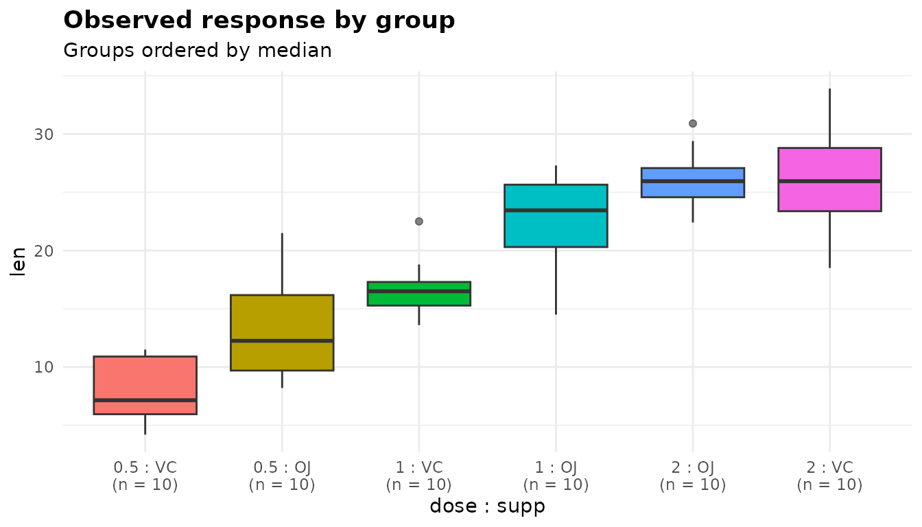

The box plot shows the observed response in each cell, ordered by median and labelled with its size. Use it to see the raw data behind the means: spreads, skewness and outliers.

plot(fit, "emmeans")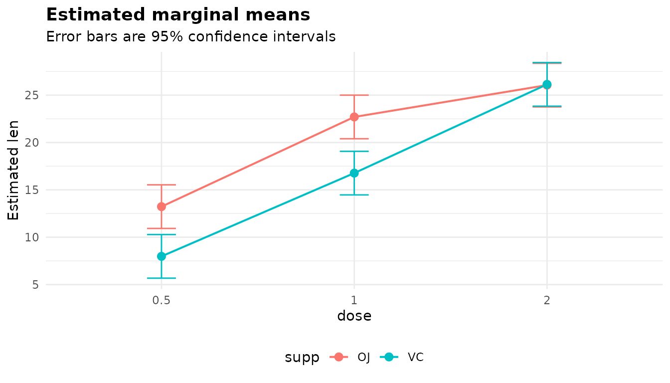

The emmeans plot shows the estimated marginal means with their 95% intervals. The first grouping factor is on the x axis and the second sets the colour, one line per supplement. Lines that are not parallel are the interaction: the gap between the supplements closes at 2 mg/day.

plot(fit, "residuals")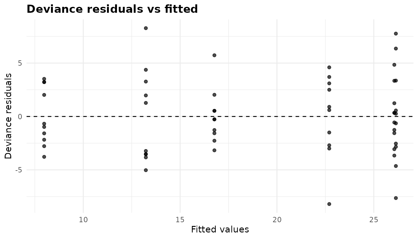

The residuals plot shows deviance residuals (for a Gaussian model, ordinary residuals) against fitted values. The points fall in vertical stripes, one per cell mean. The two 2 mg/day cells have almost the same mean, so their stripes overlap at about 26. Look for stripes of clearly different heights (unequal variances) or a funnel that widens with the fitted value (a variance that grows with the mean, which suggests another family). Here the heights vary somewhat, as the cell standard deviations did, but there is no funnel.

plot(fit, "qq")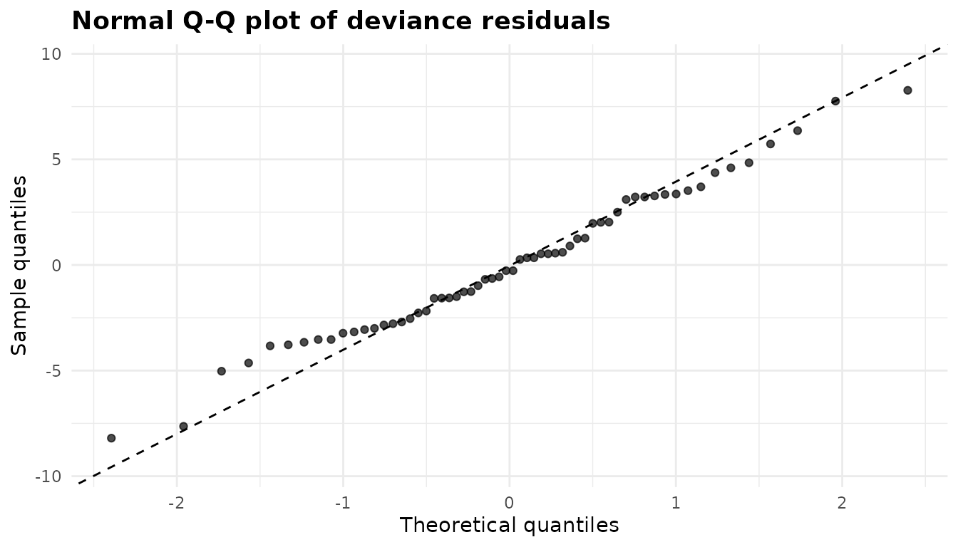

The qq plot compares the deviance residuals with a normal distribution. Points close to the dashed line support the normal-errors assumption, and systematic curvature at the ends suggests skewness or heavy tails. Here the points follow the line well. The lower tail is a little shorter than a normal one, a mild departure for a balanced design with 60 observations.

All four are ggplot2 objects that you can modify with +. See Plots and visual customisation.

A non-Gaussian family: Gamma

The data

MASS::Cars93 lists 93 car models on sale in the US in 1993. Their Price (in thousands of dollars) is positive and right-skewed, and within each Type of car the spread grows with the typical price:

cars <- MASS::Cars93[, c("Manufacturer", "Model", "Type", "Price")]
price <- split(cars$Price, cars$Type)
round(t(sapply(price, function(x) c(n = length(x), median = median(x),
                                     mean = mean(x), sd = sd(x),
                                     cv = sd(x) / mean(x)))), 2)
#>          n median  mean    sd   cv
#> Compact 16  16.15 18.21  6.69 0.37
#> Large   11  20.90 24.30  6.34 0.26
#> Midsize 22  26.20 27.22 12.26 0.45
#> Small   21  10.00 10.17  1.95 0.19
#> Sporty  14  16.80 19.39  7.97 0.41
#> Van      9  19.10 19.10  1.88 0.10

A Gaussian model assumes the same standard deviation in every group. It is about 2 for small cars and about 12 for midsize ones. A Gamma family assumes instead that the standard deviation is proportional to the mean: a constant coefficient of variation (cv). The cv column shows that fits better, though not perfectly (vans are unusually uniform). A log link makes the group effects multiplicative, so comparisons come out as ratios of means.

Fitting and the omnibus test

gam <- anova_glm(cars, "Price", "Type", family = Gamma(link = "log"))
gam
#> Analysis of deviance (Gamma family, log link, Type II) 
#> ------------------------------------------------------
#> Call: anova_glm(data = cars, response = "Price", groups = "Type", family = Gamma(link = "log"))
#> Observations used: 93
#> 
#> Omnibus test (Type II, F)
#>        term sum_sq df statistic   p_value
#> 1      Type  10.65  5     18.56 1.663e-12
#> 2 Residuals   9.98 87        NA        NA
#> 
#> Notes
#>   - McFadden's pseudo R squared is not reported (NA): the log-likelihood of a Gamma family is a log density, which shifts with the units of the response, so the ratio has no unit-free meaning. The deviance explained does not depend on the units and is reported instead.
#> 
#> Plots available: box, residuals, qq, emmeans
#>   (use plot(x, which = "box"))

family accepts a family object, as here, a family function, or a name such as "Gamma". The name alone gives the Gamma family’s default inverse link, which is rarely what you want for group comparisons (see below).

test_statistic. By default the test is chosen after fitting. A family that estimates its dispersion, like the Gaussian and the Gamma, gets an F test, and a family whose dispersion is fixed at 1 (binomial, Poisson) gets a likelihood-ratio test. In the F table of a non-Gaussian family the sum_sq column holds deviances, as the anova_glm() help page explains. The Type row is the drop in deviance when Type is added. The Residuals row is the Pearson chi-squared statistic, and dividing it by its degrees of freedom gives the dispersion. F is the ratio of the two per degree of freedom:

a <- gam$anova
(a$sum_sq[1] / a$df[1]) / (a$sum_sq[2] / a$df[2])
#> [1] 18.56058

You can ask for the likelihood-ratio or Wald statistic instead. The columns come in the same order whatever the statistic, and only an F table has sum_sq and a Residuals row:

for (ts in c("LR", "Wald")) {
  g <- anova_glm(cars, "Price", "Type", family = Gamma(link = "log"),
                 test_statistic = ts, plots = FALSE)
  cat("\n", attr(g$anova, "statistic"), "\n", sep = "")
  print(g$anova)
}
#> 
#> likelihood-ratio chi-square
#>   term df statistic      p_value
#> 1 Type  5   92.8029 1.730729e-18
#> 
#> Wald chi-square
#>   term df statistic      p_value
#> 1 Type  5  101.7011 2.314394e-20

The likelihood-ratio statistic is the deviance drop divided by the estimated dispersion, referred to a chi-squared distribution. That ignores the uncertainty in the dispersion estimate, which the F test allows for, so for a family that estimates its dispersion F is the better default. The Wald test is built from the coefficients and their covariance matrix. It is the only one of the three that can use a robust covariance (see vcov_type). Here all three agree that the car types differ.

Effect sizes

gam$effect_sizes
#>              measure estimate
#> 1 deviance_explained 0.542735
#> 2        mcfadden_r2       NA

For a non-Gaussian family there are no sums of squares, so the effect size is the deviance_explained: 1 minus the residual deviance over the null deviance. Car type explains 54% of the deviance. McFadden’s pseudo R squared is reported only for the binomial, Poisson and negative binomial families. For a Gamma model it is NA, and the note in the printout explains why.

The coefficient table and `ci_method`

co <- gam$assumptions$coefficients
co
#>          term    estimate         se  statistic      p_value distribution
#> 1 (Intercept)  2.90210817 0.08467429 34.2737820 2.652780e-52            t
#> 2   TypeLarge  0.28836818 0.13265912  2.1737532 3.243991e-02            t
#> 3 TypeMidsize  0.40177703 0.11128382  3.6103814 5.103876e-04            t
#> 4   TypeSmall -0.58299378 0.11239391 -5.1870584 1.377488e-06            t
#> 5  TypeSporty  0.06279664 0.12395047  0.5066269 6.136982e-01            t
#> 6     TypeVan  0.04758016 0.14112382  0.3371519 7.368144e-01            t
#>     conf_low  conf_high ci_method
#> 1  2.7384042  3.0752703   profile
#> 2  0.0264585  0.5545836   profile
#> 3  0.1790690  0.6219030   profile
#> 4 -0.8077507 -0.3604911   profile
#> 5 -0.1832054  0.3101515   profile
#> 6 -0.2297083  0.3322378   profile

The coefficients are on the log scale. The intercept is the log of the mean price of the reference type, Compact, and each other coefficient is the log of a ratio to it: small cars cost exp(-0.583) = 0.56 times as much as compact ones on average. The distribution column says the tests use t, because the dispersion is estimated.

ci_method = "profile" (the default) gives profile-likelihood intervals, cut at t quantiles so that they agree with the t tests beside them. ci_method = "wald" gives estimate ± t × SE:

wald <- anova_glm(cars, "Price", "Type", family = Gamma(link = "log"),
                  ci_method = "wald", plots = FALSE)$assumptions$coefficients
cbind(co[, c("term", "estimate")],
      profile = co[, c("conf_low", "conf_high")],
      wald = wald[, c("conf_low", "conf_high")])
#>          term    estimate profile.conf_low profile.conf_high wald.conf_low
#> 1 (Intercept)  2.90210817        2.7384042         3.0752703    2.73380885
#> 2   TypeLarge  0.28836818        0.0264585         0.5545836    0.02469382
#> 3 TypeMidsize  0.40177703        0.1790690         0.6219030    0.18058839
#> 4   TypeSmall -0.58299378       -0.8077507        -0.3604911   -0.80638884
#> 5  TypeSporty  0.06279664       -0.1832054         0.3101515   -0.18356834
#> 6     TypeVan  0.04758016       -0.2297083         0.3322378   -0.23291870
#>   wald.conf_high
#> 1      3.0704075
#> 2      0.5520425
#> 3      0.6229657
#> 4     -0.3595987
#> 5      0.3091616
#> 6      0.3280790

The two differ in the third decimal place here. Profile intervals follow the shape of the likelihood, which matters more in small samples or near a boundary. Wald intervals are symmetric on the log scale. Exponentiate either to get an interval for the ratio.

Dispersion

gam$assumptions$dispersion
#> [1] 0.1147158
sqrt(gam$assumptions$dispersion)
#> [1] 0.3386972

For a Gamma family the dispersion is the squared coefficient of variation. The model therefore puts the standard deviation of prices at about 34% of the mean in every car type. The observed values above range from 10% (vans) to 45% (midsize cars), so the constant-CV assumption is only roughly true. The vcov_type section shows how to make the comparisons robust to that.

`$model_stats` and `$family`

str(gam$model_stats)
#> List of 5
#>  $ AIC              : num 595
#>  $ BIC              : num 613
#>  $ null_deviance    : num 19.6
#>  $ residual_deviance: num 8.97
#>  $ df_residual      : int 87
gam$family
#> 
#> Family: Gamma 
#> Link function: log

$model_stats holds the AIC, BIC, null and residual deviances and residual degrees of freedom. $family is the family object actually used. Because the Gaussian and Gamma fits are full likelihoods for the same response, their AICs can be compared directly:

gau <- anova_glm(cars, "Price", "Type", plots = FALSE)
c(gaussian = gau$model_stats$AIC, gamma = gam$model_stats$AIC)
#> gaussian    gamma 
#> 651.4658 594.8847

The Gamma model is much better supported.

Marginal means on the response scale

gam$emmeans
#>      Type estimate        se df  conf_low conf_high
#> 1 Compact 18.21250 1.5421305 87 15.391399  21.55068
#> 2   Large 24.30000 2.4815412 87 19.836025  29.76856
#> 3 Midsize 27.21818 1.9654379 87 23.579061  31.41895
#> 4   Small 10.16667 0.7514161 87  8.777667  11.77546
#> 5  Sporty 19.39286 1.7554535 87 16.199579  23.21560
#> 6     Van 19.10000 2.1563719 87 15.260827  23.90499

The marginal means are on the response scale, in thousands of dollars. In a one-factor model they are the group means. Their intervals are computed on the log scale and back-transformed, so they are not symmetric about the estimate.

With a log link, a pairwise comparison is a ratio of means, in a column called ratio, tested against a null value of 1:

gph <- gam$posthoc
print(gph[gph$p_adjusted < 0.05,
          c("contrast", "ratio", "conf_low", "conf_high", "p_adjusted")],
      digits = 3)
#>             contrast ratio conf_low conf_high p_adjusted
#> 2  Compact / Midsize 0.669    0.484     0.925   6.57e-03
#> 3    Compact / Small 1.791    1.291     2.486   2.00e-05
#> 7      Large / Small 2.390    1.655     3.451   1.16e-08
#> 10   Midsize / Small 2.677    1.981     3.618   3.09e-10
#> 11  Midsize / Sporty 1.404    1.002     1.967   4.83e-02
#> 13    Small / Sporty 0.524    0.373     0.737   4.94e-06
#> 14       Small / Van 0.532    0.359     0.789   1.53e-04

Those are the comparisons that survive Tukey’s adjustment. Midsize cars, for example, average 2.68 times the price of small ones.

The link decides what a comparison is

With the log link comparisons are ratios, and with the logit link they are odds ratios. With any other non-identity link they are differences between the means on the response scale, and $notes says so. The Gamma family’s default link is the inverse:

inv <- anova_glm(cars, "Price", "Type", family = "Gamma", plots = FALSE)
inv$method
#> [1] "Analysis of deviance (Gamma family, inverse link, Type II)"
inv$notes[grepl("link", inv$notes)]
#> [1] "With the inverse link the pairwise comparisons are differences between the marginal means on the response scale; only log and logit links give ratios."
head(inv$posthoc[, c("contrast", "estimate", "conf_low", "conf_high")], 3)
#>            contrast  estimate   conf_low conf_high
#> 1   Compact - Large -6.087500 -14.601888  2.426888
#> 2 Compact - Midsize -9.005682 -16.286022 -1.725342
#> 3   Compact - Small  8.045833   3.046632 13.045035

Plots for the Gamma fit

plot(gam, "residuals")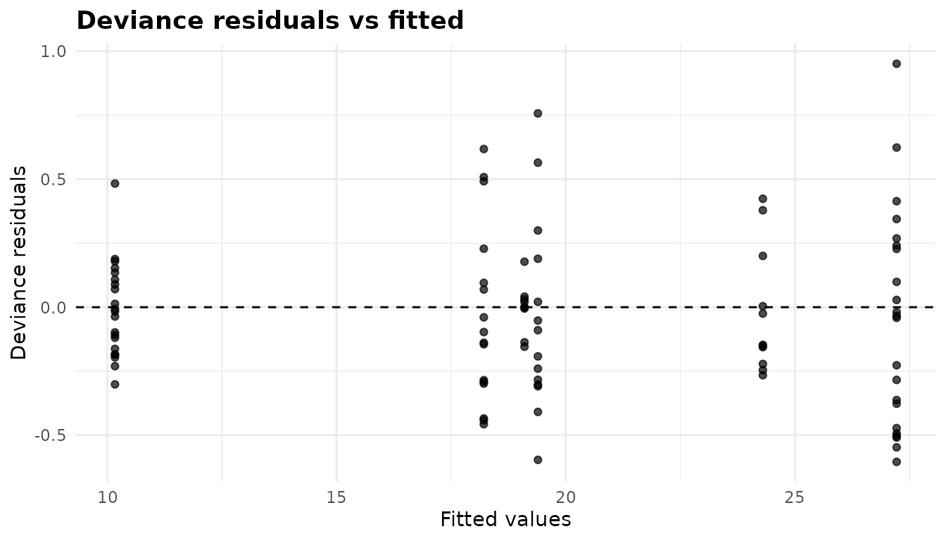

If the variance really is proportional to the mean squared, the deviance residuals of a Gamma model have roughly the same spread at every fitted value. Here the stripes differ in height. Two sit side by side at about 19: vans (19.1) on the left and sporty cars (19.4) on the right. The vans’ stripe is by far the shortest, because their prices vary much less than the model assumes. The midsize stripe, at about 27, is the tallest.

plot(gam, "qq")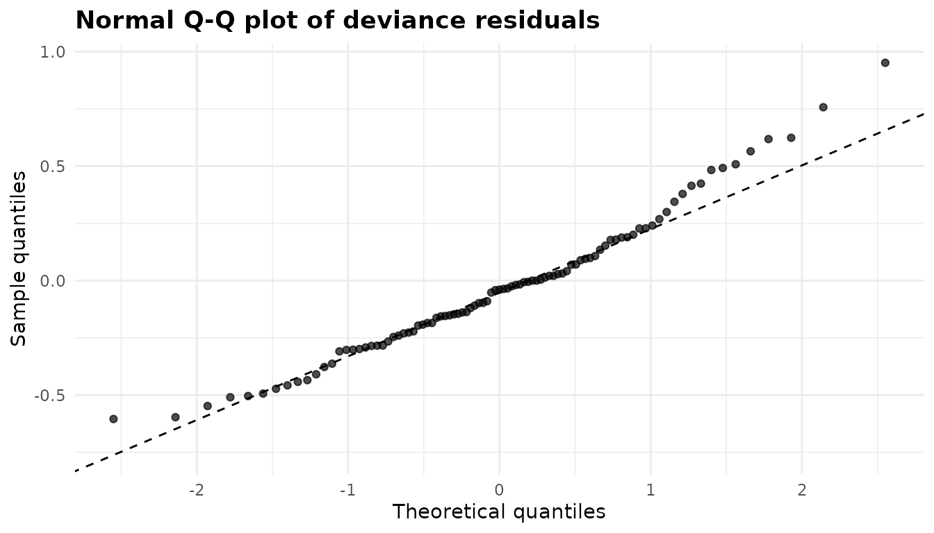

The deviance residuals of a Gamma model are approximately normal when the model fits. Here the middle follows the line and the upper tail rises above it: a few cars are dearer than a Gamma distribution with this dispersion would suggest. gam$model is an ordinary glm, so you can find them directly:

res <- residuals(gam$model, type = "deviance")
head(cars[order(res, decreasing = TRUE), ], 3)
#>     Manufacturer    Model    Type Price
#> 59 Mercedes-Benz     300E Midsize  61.9
#> 19     Chevrolet Corvette  Sporty  38.0
#> 48      Infiniti      Q45 Midsize  47.9

plot(gam, "emmeans")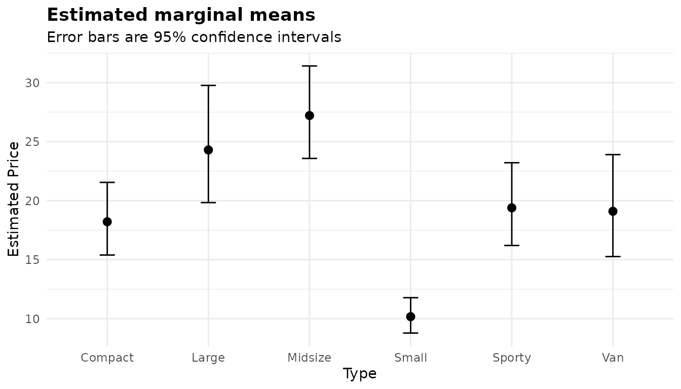

The emmeans plot shows the means on the response scale, with their asymmetric intervals. Type has no natural order, so the points are not joined by a line. Lines appear only across a second grouping factor, as in the ToothGrowth plot, or along an ordered factor on the x axis. plot(gam, "box") shows the raw prices by type, as for the Gaussian fit.

Options worth knowing

`vcov_type`: robust standard errors

vcov_type takes an HC type ("HC0" to "HC4") from the sandwich package. The robust covariance does not rely on the family’s variance function, so it protects the marginal means and comparisons when that function is wrong, as the vans suggest it is here:

rob <- anova_glm(cars, "Price", "Type", family = Gamma(link = "log"),
                 vcov_type = "HC3", plots = FALSE)
cbind(rob$emmeans[, "Type", drop = FALSE],
      se_model = gam$emmeans$se, se_HC3 = rob$emmeans$se)
#>      Type  se_model    se_HC3
#> 1 Compact 1.5421305 1.7265476
#> 2   Large 2.4815412 2.0040958
#> 3 Midsize 1.9654379 2.6764077
#> 4   Small 0.7514161 0.4367684
#> 5  Sporty 1.7554535 2.2117883
#> 6     Van 2.1563719 0.6640312
rob$notes
#> [1] "The omnibus F test compares deviances, so it rests on the model-based variance; the robust (HC3) covariance is used only by the coefficient table, the marginal means and the comparisons. For an omnibus test that uses it, set test_statistic = \"Wald\"."              
#> [2] "McFadden's pseudo R squared is not reported (NA): the log-likelihood of a Gamma family is a log density, which shifts with the units of the response, so the ratio has no unit-free meaning. The deviance explained does not depend on the units and is reported instead."
#> [3] "Robust standard errors (HC3) were requested, so the coefficient intervals are Wald intervals built from them; profile-likelihood intervals cannot use a sandwich covariance."

The standard error for vans shrinks and the one for midsize cars grows: each now reflects that type’s own spread. The notes spell out where the robust covariance is used. It goes into the coefficient table (with Wald intervals, since profile intervals cannot use it), the marginal means and the comparisons. The omnibus F test compares deviances and cannot use it. To make the omnibus test robust too, set test_statistic = "Wald":

anova_glm(cars, "Price", "Type", family = Gamma(link = "log"),
          vcov_type = "HC3", test_statistic = "Wald", plots = FALSE)$anova
#>   term df statistic      p_value
#> 1 Type  5  195.7549 2.298221e-40

`weights`

weights names a column of prior weights. It is given as a column name, not a vector, so the weights are subsetted with the data and cannot misalign when a row is dropped. A natural use with the Gamma family is a response that is itself an average. The mean of m prices has variance φμ²/m, so its prior weight is m. Suppose you had only the average price per manufacturer and type, with the number of models behind each average:

agg <- aggregate(Price ~ Manufacturer + Type, data = cars, FUN = mean)
agg$n_models <- aggregate(Price ~ Manufacturer + Type, data = cars,
                          FUN = length)$Price
nrow(agg)
#> [1] 81
table(agg$n_models)
#> 
#>  1  2 
#> 69 12

Weighting each average by its count recovers the means of the full data exactly. Ignoring the counts does not:

w_fit <- anova_glm(agg, "Price", "Type", family = Gamma(link = "log"),
                   weights = "n_models", plots = FALSE)
u_fit <- anova_glm(agg, "Price", "Type", family = Gamma(link = "log"),
                   plots = FALSE)
data.frame(Type = gam$emmeans$Type, full_data = gam$emmeans$estimate,
           weighted = w_fit$emmeans$estimate,
           unweighted = u_fit$emmeans$estimate)
#>      Type full_data weighted unweighted
#> 1 Compact  18.21250 18.21250   18.60000
#> 2   Large  24.30000 24.30000   24.50500
#> 3 Midsize  27.21818 27.21818   27.31000
#> 4   Small  10.16667 10.16667   10.36875
#> 5  Sporty  19.39286 19.39286   19.16667
#> 6     Van  19.10000 19.10000   19.43125

The standard errors differ slightly from the full-data fit, because the dispersion is now estimated from 81 averages rather than 93 cars.

A row with a weight of zero contributes nothing to the fit, so it is dropped before fitting, counted in $n_removed and named in $notes:

agg0 <- agg
agg0$n_models[1] <- 0
z_fit <- anova_glm(agg0, "Price", "Type", family = Gamma(link = "log"),
                   weights = "n_models", plots = FALSE)
z_fit$n_removed
#> [1] 1
z_fit$notes[1]
#> [1] "Dropped 1 row(s) whose weight in `n_models` is zero: they contribute nothing to the fit, and keeping them would make row counts, robust standard errors and information criteria disagree with it."

`interaction`

The default, interaction = FALSE, fits the grouping factors additively. The marginal means and comparisons are then reported for each factor on its own, averaged over the others, with a term column saying which, and each factor’s comparisons form their own multiplicity family:

add <- anova_glm(tg, "len", c("dose", "supp"), plots = FALSE)
add$emmeans
#>   term dose supp estimate        se df  conf_low conf_high
#> 1 dose  0.5 <NA> 10.60500 0.8558752 56  8.890476  12.31952
#> 2 dose    1 <NA> 19.73500 0.8558752 56 18.020476  21.44952
#> 3 dose    2 <NA> 26.10000 0.8558752 56 24.385476  27.81452
#> 4 supp <NA>   OJ 20.66333 0.6988192 56 19.263430  22.06324
#> 5 supp <NA>   VC 16.96333 0.6988192 56 15.563430  18.36324
add$notes
#> [1] "The grouping factors enter the model additively, so $emmeans and $posthoc are reported for each factor separately, averaged over the others (column `term`), and each factor's comparisons are a separate multiplicity family. Set interaction = TRUE to compare cells instead."

interaction = TRUE fits the full factorial. With three or more factors a whole number sets the highest order of interaction: interaction = 2 keeps the two-way interactions and drops the rest.

`adjust` and `conf_level`

adjust is applied by emmeans and accepts "tukey" (the default), "sidak", "scheffe", "dunnettx", "bonferroni", "holm", "hochberg", "hommel", "BH", "BY", "fdr" or "none". A step-down method such as Holm cannot be turned into intervals, so emmeans uses Bonferroni intervals beside Holm p-values, and $notes says so:

holm <- anova_glm(tg, "len", c("dose", "supp"), interaction = TRUE,
                  adjust = "holm", plots = FALSE)
holm$notes
#> [1] "The comparison intervals use the bonferroni adjustment while the p-values use holm: emmeans cannot turn holm into intervals."

conf_level sets the level of every interval: the coefficient table, the marginal means and the comparisons.

What the notes say

fit$notes
#> character(0)
gam$notes
#> [1] "McFadden's pseudo R squared is not reported (NA): the log-likelihood of a Gamma family is a log density, which shifts with the units of the response, so the ratio has no unit-free meaning. The deviance explained does not depend on the units and is reported instead."

The ToothGrowth fit has no notes. No rows were dropped, the model is far from saturated, nothing failed to compute, and the Gaussian family has partial eta squared to report. The Gamma fit has one, explaining why McFadden’s pseudo R squared is NA. Other notes you have seen above: the robust covariance and where it is used, the per-factor reporting of an additive model, Bonferroni intervals beside Holm p-values, and differences rather than ratios under the inverse link. Read $notes on every fit.

Reporting the result

Write-ups built from the fits with inline R, so the numbers cannot drift from the analysis:

A two-way analysis of variance (Type II) found that odontoblast length depended on the dose of vitamin C, F(2, 54) = 92.00, p < 0.001, partial η² = 0.77, and on the supplement, F(1, 54) = 15.57, p < 0.001, with an interaction between them, F(2, 54) = 4.11, p = 0.022. Orange juice produced longer odontoblasts than ascorbic acid at 0.5 mg/day (difference 5.25, Tukey-adjusted p = 0.024) and 1 mg/day (5.93, adjusted p = 0.007), but not at 2 mg/day (-0.08, adjusted p = 1.000).

In a Gamma model with a log link, car prices differed by type, F(5, 87) = 18.56, p < 0.001, with type explaining 54% of the deviance. Midsize cars cost 2.68 times as much as small cars on average (95% CI 1.98 to 3.62, Tukey-adjusted).

For a model on a non-identity link, say which family and link you used, and report comparisons in the form they take on it: ratios for a log link.

The data

Fitting the model

The omnibus test

Type II or Type III

Effect sizes

Marginal means and comparisons

Checking assumptions

Plots

A non-Gaussian family: Gamma

The data

Fitting and the omnibus test

Effect sizes

The coefficient table and ci_method

Dispersion

$model_stats and $family

Marginal means on the response scale

The link decides what a comparison is

Plots for the Gamma fit

Options worth knowing

vcov_type: robust standard errors

weights

interaction

adjust and conf_level

What the notes say

Reporting the result

See also

The coefficient table and `ci_method`

`$model_stats` and `$family`

`vcov_type`: robust standard errors

`weights`

`interaction`

`adjust` and `conf_level`