Every anovakit function returns an object of class
anovakit_fit. It is a plain named list: every table is a
data frame, every figure a ggplot2 object, and nothing
is hidden behind accessor functions. This article shows what is in it
and how to use it. The examples use chickwts, the weights
of 71 chicks raised on six feed supplements.
table(chickwts$feed)
#>
#>    casein horsebean   linseed  meatmeal   soybean sunflower
#>        12        10        12        11        14        12
fit <- anova_glm(chickwts, "weight", "feed")anova_glm() with its default Gaussian family is a
classical one-way ANOVA, which is a convenient model-based example.
Everything below applies to all eight functions; where one differs, it
says so.
What is in a fit
class(fit)
#> [1] "anovakit_fit"
names(fit)
#>  [1] "method"         "call"           "model"          "anova"
#>  [5] "effect_sizes"   "emmeans"        "emmeans_object" "posthoc"
#>  [9] "assumptions"    "plots"          "data_used"      "n_removed"
#> [13] "conf_level"     "notes"          "family"         "model_stats"
The first fourteen components are the same for every function:
| Component | What it holds |
|---|---|
method |
The analysis that was run, as printed. |
call |
The call that made the fit. |
model |
The fitted model (lm, glm,
mlm, afex_aov), or the htest for
anova_welch() and anova_kw(). |
anova |
The omnibus test table. |
effect_sizes |
The method’s effect sizes, with intervals where they exist. |
emmeans |
Estimated marginal means (group summaries for Welch and Kruskal-Wallis). |
emmeans_object |
The emmeans grid behind $emmeans, for
further contrasts. |
posthoc |
Pairwise comparisons. |
assumptions |
The assumption checks this method needs. |
plots |
Named list of ggplot2 figures. |
data_used |
The rows and columns the analysis actually used. |
n_removed |
How many input rows are not in data_used. |
conf_level |
The level of every interval in the fit. |
notes |
Everything the function decided or could not compute. |
After those come the components a function adds for itself: here
family and model_stats.
anova_ancova() adds the slopes test and the simple slopes,
anova_rm() the sphericity table and the subjects it
dropped, and so on. Each walkthrough describes its own, and
?anovakit_fit lists them all.
Printing
print() shows the omnibus table, any notes, and the
names of the plots:
fit
#> Analysis of deviance (gaussian family, identity link, Type II)
#> --------------------------------------------------------------
#> Call: anova_glm(data = chickwts, response = "weight", groups = "feed")
#> Observations used: 71
#>
#> Omnibus test (Type II, F)
#>        term sum_sq df statistic   p_value
#> 1      feed 231100  5     15.36 5.936e-10
#> 2 Residuals 195600 65        NA        NA
#>
#> Plots available: box, residuals, qq, emmeans
#>   (use plot(x, which = "box"))
summary() shows the rest: effect sizes, marginal means,
comparisons and the assumption checks. It returns an object, so you can
keep it and print it later with different digits.
s <- summary(fit, digits = 3)
class(s)
#> [1] "summary.anovakit_fit"
s
#> Analysis of deviance (gaussian family, identity link, Type II)
#> --------------------------------------------------------------
#> Call: anova_glm(data = chickwts, response = "weight", groups = "feed")
#> Observations used: 71
#>
#> Omnibus test (Type II, F)
#>        term sum_sq df statistic  p_value
#> 1      feed 231000  5      15.4 5.94e-10
#> 2 Residuals 196000 65        NA       NA
#>
#> Plots available: box, residuals, qq, emmeans
#>   (use plot(x, which = "box"))
#>
#> Assumption checks
#>
#>   dispersion
#>     3010
#>
#>   coefficients
#>           term estimate   se statistic  p_value distribution conf_low conf_high
#>    (Intercept)   324.00 15.8    20.400  < 2e-16            t    292.0   355.000
#>  feedhorsebean  -163.00 23.5    -6.960 2.07e-09            t   -210.0  -116.000
#>    feedlinseed  -105.00 22.4    -4.680 1.49e-05            t   -150.0   -60.100
#>   feedmeatmeal   -46.70 22.9    -2.040 0.045567            t    -92.4    -0.948
#>    feedsoybean   -77.20 21.6    -3.580 0.000665            t   -120.0   -34.100
#>  feedsunflower     5.33 22.4     0.238 0.812495            t    -39.4    50.100
#>  ci_method
#>    profile
#>    profile
#>    profile
#>    profile
#>    profile
#>    profile
#>
#> Effect sizes
#>  term df sum_sq partial_eta_sq partial_omega_sq
#>  feed  5 231000          0.542            0.503
#>
#> Estimated marginal means (95% intervals)
#>       feed estimate   se df conf_low conf_high
#>     casein      324 15.8 65      292       355
#>  horsebean      160 17.3 65      126       195
#>    linseed      219 15.8 65      187       250
#>   meatmeal      277 16.5 65      244       310
#>    soybean      246 14.7 65      217       276
#>  sunflower      329 15.8 65      297       361
#>
#> Pairwise comparisons
#>               contrast estimate   se df conf_low conf_high statistic  p_value
#>     casein - horsebean   163.00 23.5 65     94.4    232.00     6.960 2.07e-09
#>       casein - linseed   105.00 22.4 65     39.1    171.00     4.680 1.49e-05
#>      casein - meatmeal    46.70 22.9 65    -20.6    114.00     2.040 0.045567
#>       casein - soybean    77.20 21.6 65     13.8    141.00     3.580 0.000665
#>     casein - sunflower    -5.33 22.4 65    -71.1     60.40    -0.238 0.812495
#>    horsebean - linseed   -58.60 23.5 65   -128.0     10.40    -2.490 0.015222
#>   horsebean - meatmeal  -117.00 24.0 65   -187.0    -46.30    -4.870 7.48e-06
#>    horsebean - soybean   -86.20 22.7 65   -153.0    -19.50    -3.800 0.000325
#>  horsebean - sunflower  -169.00 23.5 65   -238.0    -99.80    -7.180 8.20e-10
#>     linseed - meatmeal   -58.20 22.9 65   -125.0      9.07    -2.540 0.013479
#>      linseed - soybean   -27.70 21.6 65    -91.0     35.70    -1.280 0.204145
#>    linseed - sunflower  -110.00 22.4 65   -176.0    -44.40    -4.920 6.21e-06
#>     meatmeal - soybean    30.50 22.1 65    -34.4     95.40     1.380 0.172554
#>   meatmeal - sunflower   -52.00 22.9 65   -119.0     15.20    -2.270 0.026435
#>    soybean - sunflower   -82.50 21.6 65   -146.0    -19.10    -3.820 0.000298
#>  p_adjusted adjustment
#>    3.07e-08      tukey
#>    0.000210      tukey
#>    0.332458      tukey
#>    0.008365      tukey
#>    0.999890      tukey
#>    0.141333      tukey
#>    0.000106      tukey
#>    0.004217      tukey
#>    1.22e-08      tukey
#>    0.127696      tukey
#>    0.793285      tukey
#>    8.84e-05      tukey
#>    0.739136      tukey
#>    0.220696      tukey
#>    0.003885      tukey
Both use digits for display only; the numbers stored in
the fit are never rounded.
The tables are ordinary data frames
Every table is a data frame with a documented column layout, so base R, dplyr or data.table all work on it without conversion.
fit$anova
#>        term   sum_sq df statistic     p_value
#> 1      feed 231129.2  5   15.3648 5.93642e-10
#> 2 Residuals 195556.0 65        NA          NA
The model-based functions attach the test details to the omnibus
table as attributes, which is how print() knows what
heading to write:
attributes(fit$anova)[c("ss_type", "statistic")]
#> $ss_type
#> [1] "II"
#>
#> $statistic
#> [1] "F"
The pairwise comparisons have one row per pair. p_value
is the unadjusted p-value, p_adjusted the adjusted
one, and adjustment names the method, so nothing about the
adjustment has to be remembered from the call:
names(fit$posthoc)
#>  [1] "contrast"   "estimate"   "se"         "df"         "conf_low"
#>  [6] "conf_high"  "statistic"  "p_value"    "p_adjusted" "adjustment"
unique(fit$posthoc$adjustment)
#> [1] "tukey"
Selecting and sorting is plain subsetting. Here are the comparisons that survive the Tukey adjustment, largest difference first:
ph <- fit$posthoc
sig <- ph[ph$p_adjusted < 0.05, c("contrast", "estimate", "conf_low",
                                  "conf_high", "p_adjusted")]
sig[order(-abs(sig$estimate)), ]
#>                 contrast   estimate   conf_low conf_high   p_adjusted
#> 9  horsebean - sunflower -168.71667 -237.68021 -99.75312 1.219887e-08
#> 1     casein - horsebean  163.38333   94.41979 232.34688 3.070197e-08
#> 7   horsebean - meatmeal -116.70909 -187.08308 -46.33510 1.062092e-04
#> 12   linseed - sunflower -110.16667 -175.92082 -44.41251 8.843233e-05
#> 2       casein - linseed  104.83333   39.07918 170.58749 2.100151e-04
#> 8    horsebean - soybean  -86.22857 -152.91546 -19.54168 4.216654e-03
#> 15   soybean - sunflower  -82.48810 -145.85039 -19.12580 3.884521e-03
#> 4       casein - soybean   77.15476   13.79247 140.51705 8.365309e-03
The intervals in $posthoc from the model-based functions
are simultaneous. With a single-step method such as Tukey’s they use the
same adjustment as p_adjusted, so an interval that excludes
zero agrees with an adjusted p-value below 1 - conf_level.
Step-down methods such as Holm’s cannot be turned into intervals;
emmeans then uses Bonferroni intervals, and
$notes says so.
Writing a table out is one line:
write.csv(fit$posthoc, "comparisons.csv", row.names = FALSE)Read the notes
$notes is a character vector. It records every decision
the function made on your behalf (which model it chose, which rows it
dropped, which correction it applied), everything it could not compute
and why, and anything car, emmeans,
stats or afex said while fitting. None
of it is printed to the console as a warning, so this is the one place
to look.
This simple fit needed no decisions, so its notes are empty:
fit$notes
#> character(0)
Ask for heteroscedasticity-consistent standard errors and there is more to say: which parts of the output use them, and what they cannot do.
robust <- anova_glm(chickwts, "weight", "feed", vcov_type = "HC3",
                    plots = FALSE)
writeLines(robust$notes)
#> Comparisons that use robust standard errors keep the residual degrees of freedom of the model; with very small groups of unequal variance they can be anti-conservative, and for a one-way design anova_welch() is better calibrated.
#> The omnibus F test compares deviances, so it rests on the model-based variance; the robust (HC3) covariance is used only by the coefficient table, the marginal means and the comparisons. For an omnibus test that uses it, set test_statistic = "Wald".
#> Robust standard errors (HC3) were requested, so the coefficient intervals are Wald intervals built from them; profile-likelihood intervals cannot use a sandwich covariance.
Treat the notes as a checklist to read before you quote a number. They are plain text, so you can also search them, for example to flag which fits in a batch used robust standard errors:
fits <- list(
  welch  = anova_welch(chickwts, "weight", "feed", plots = FALSE),
  glm    = fit,
  robust = robust
)
vapply(fits, function(f) length(f$notes), integer(1))
#>  welch    glm robust
#>      0      0      3
vapply(fits, function(f) any(grepl("robust", f$notes, ignore.case = TRUE)),
       logical(1))
#>  welch    glm robust
#>  FALSE  FALSE   TRUE
Which rows were used
Every function drops rows it cannot analyse (missing or infinite
values in the analysed columns, zero weights, and in
anova_rm() subjects with an incomplete design) and counts
them. nrow(fit$data_used) + fit$n_removed is always the
number of rows you supplied:
gappy <- chickwts
gappy$weight[c(3, 17, 40)] <- NA
g <- anova_glm(gappy, "weight", "feed", plots = FALSE)
c(supplied = nrow(gappy), used = nrow(g$data_used), removed = g$n_removed)
#> supplied     used  removed
#>       71       68        3
$data_used holds only the analysed columns, in the form
the model saw them: grouping columns as factors, and covariates
mean-centred when anova_ancova() or
anova_manova() centred them.
str(g$data_used)
#> 'data.frame':    68 obs. of  2 variables:
#>  $ weight: num  179 160 227 217 168 108 124 143 140 309 ...
#>  $ feed  : Factor w/ 6 levels "casein","horsebean",..: 2 2 2 2 2 2 2 2 2 3 ...
Going further with emmeans
$emmeans and $posthoc cover the usual
questions: the mean of each group, and every pairwise difference. For
anything else, $emmeans_object is the
emmeans reference grid the tables were built from.
grid <- fit$emmeans_object
class(grid)
#> [1] "emmGrid"
#> attr(,"package")
#> [1] "emmeans"
For example, comparing every feed with horsebean
(Dunnett-style comparisons with a control) instead of all 15 pairs:
ct <- emmeans::contrast(grid, "trt.vs.ctrl", ref = "horsebean")
confint(ct, level = fit$conf_level)
#>  contrast              estimate   SE df lower.CL upper.CL
#>  casein - horsebean       163.4 23.5 65    102.5      224
#>  linseed - horsebean       58.5 23.5 65     -2.3      119
#>  meatmeal - horsebean     116.7 24.0 65     54.6      179
#>  soybean - horsebean       86.2 22.7 65     27.4      145
#>  sunflower - horsebean    168.7 23.5 65    107.9      230
#>
#> Degrees-of-freedom method: user-specified
#> Confidence level used: 0.95
#> Conf-level adjustment: dunnettx method for 5 estimates
Or a custom contrast: the four plant-based feeds against the two animal-based ones. The coefficients follow the order of the factor levels.
levels(chickwts$feed)
#> [1] "casein"    "horsebean" "linseed"   "meatmeal"  "soybean"   "sunflower"
plant_vs_animal <- list(
  "plant - animal" = c(casein = -1/2, horsebean = 1/4, linseed = 1/4,
                       meatmeal = -1/2, soybean = 1/4, sunflower = 1/4)
)
confint(emmeans::contrast(grid, plant_vs_animal), level = fit$conf_level)
#>  contrast       estimate SE df lower.CL upper.CL
#>  plant - animal    -61.7 14 65    -89.5    -33.8
#>
#> Degrees-of-freedom method: user-specified
#> Confidence level used: 0.95
Two things to keep in mind:
- The grid carries emmeans’ default confidence level,
not the fit’s
conf_level. Passlevel = fit$conf_level(as above) when you want the two to agree. - When grouping factors enter a model additively, the means are
reported per factor and
$emmeans_objectis a named list with one grid per factor. Inanova_manova()there is one grid per response, underfit$univariate[[response]]$emmeans_object.anova_welch()andanova_kw()fit no model emmeans can use, so theirs isNULL.
Going further with the model
$model is the fitted model itself: an lm,
glm, negbin, multivariate mlm or
afex_aov. Its call refers to the analysed rows through an
environment the fit carries, so the usual model functions work on it
directly, from anywhere:
class(fit$model)
#> [1] "glm" "lm"
null <- update(fit$model, . ~ 1)
anova(null, fit$model, test = "F")
#> Analysis of Deviance Table
#>
#> Model 1: weight ~ 1
#> Model 2: weight ~ feed
#>   Resid. Df Resid. Dev Df Deviance      F    Pr(>F)
#> 1        70     426685
#> 2        65     195556  5   231129 15.365 5.936e-10 ***
#> ---
#> Signif. codes:  0 '***' 0.001 '**' 0.01 '*' 0.05 '.' 0.1 ' ' 1
AIC(null, fit$model)
#>           df      AIC
#> null       2 823.2689
#> fit$model  7 777.8748
anova_welch() and anova_kw() fit no model;
for them $model is the htest returned by
oneway.test() or kruskal.test().
fits$welch$model
#>
#>  One-way analysis of means (not assuming equal variances)
#>
#> data:  weight and feed
#> F = 19.662, num df = 5.000, denom df = 29.952, p-value = 1.177e-08
Plots
$plots is a named list of ggplot2 objects, built but
never drawn. plot(fit, "name") returns one, and
plot(fit) returns the first:
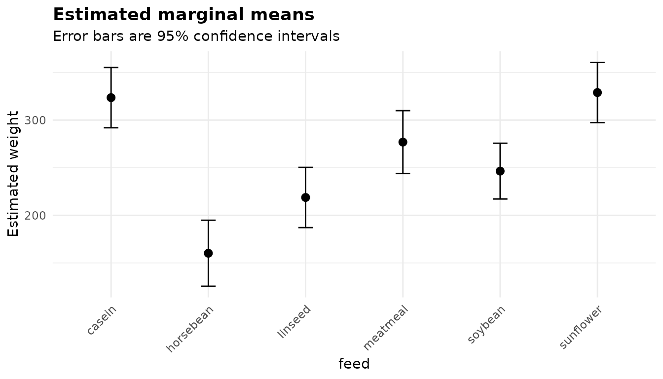
They are ordinary ggplot2 objects, so + adds to them.
The plots guide shows every figure the
package makes and how to customise it. When you are fitting many models
and do not need the figures, plots = FALSE skips building
them and keeps the objects small.
Many analyses at once
Because every function has the same signature and returns the same
structure, running one analysis over several outcomes or subsets is a
loop. Here the built-in ToothGrowth data compare the two
vitamin C supplements separately at each dose:
tg <- ToothGrowth
by_dose <- lapply(split(tg, tg$dose), function(d) {
  anova_welch(d, "len", "supp", plots = FALSE)
})
data.frame(
  dose      = names(by_dose),
  statistic = vapply(by_dose, function(f) f$anova$statistic, numeric(1)),
  df        = vapply(by_dose, function(f) f$anova$den_df, numeric(1)),
  p_value   = vapply(by_dose, function(f) f$anova$p_value, numeric(1)),
  row.names = NULL
)
#>   dose   statistic       df     p_value
#> 1  0.5 10.04720592 14.96875 0.006358607
#> 2    1 16.26323092 15.35767 0.001038376
#> 3    2  0.00212854 14.03982 0.963851589
If you then need to adjust across those tests,
p.adjust() on the p_value column does it.
Reporting a result
Everything a write-up needs is in the tables. A small helper keeps the formatting in one place:
fmt_p <- function(p) {
  if (p < 0.001) "p < .001" else sprintf("p = %s", sub("^0", "", sprintf("%.3f", p)))
}
a <- fit$anova[fit$anova$term == "feed", ]
res_df <- fit$anova$df[fit$anova$term == "Residuals"]
es <- fit$effect_sizes[fit$effect_sizes$term == "feed", ]
es
#>   term df   sum_sq partial_eta_sq partial_omega_sq
#> 1 feed  5 231129.2      0.5416855        0.5028847
Chick weight differed between feed supplements, F(5, 65) = 15.36, p < .001, partial η² = 0.54, partial ω² = 0.50. Of the 15 pairwise comparisons, 8 were significant after Tukey’s adjustment.
Because the numbers come from the fit rather than being typed, they cannot drift from the analysis when the data change.
Saving and reproducing
A fit is an ordinary R object, so saveRDS() stores it
whole, figures included. $call records how it was made:
fit$call
#> anova_glm(data = chickwts, response = "weight", groups = "feed")
Fits made with plots = FALSE are much smaller, which
matters when you store many of them.