Welch's ANOVA: comparing means when variances differ

library(anovakit)

anova_welch() compares the mean of a numeric response across two or more groups without assuming that the groups share a variance. It is the package’s default choice for a one-way comparison of means: when the variances are equal it gives up almost nothing to the classical F test, and when they are not it keeps its stated error rate where the classical test does not. If the response is heavily skewed, ordinal, or has values that are only “more extreme” rather than measured, compare ranks with anova_kw() (walkthrough). To adjust for a covariate use anova_ancova(), and to separate the main effects and interaction of two or more factors use anova_glm() (walkthrough). The decision guide covers the choice in more detail.

The data

PlantGrowth records the dried weight of 30 plants, ten grown under control conditions and ten under each of two treatments.

head(PlantGrowth)
#>   weight group
#> 1   4.17  ctrl
#> 2   5.58  ctrl
#> 3   5.18  ctrl
#> 4   6.11  ctrl
#> 5   4.50  ctrl
#> 6   4.61  ctrl
table(PlantGrowth$group)
#> 
#> ctrl trt1 trt2 
#>   10   10   10
sds <- tapply(PlantGrowth$weight, PlantGrowth$group, sd)
round(cbind(mean = tapply(PlantGrowth$weight, PlantGrowth$group, mean),
            sd = sds), 3)
#>       mean    sd
#> ctrl 5.032 0.583
#> trt1 4.661 0.794
#> trt2 5.526 0.443

The question is whether the treatments change the mean weight. The standard deviations are not the same: trt1 varies about 1.79 times as much as trt2, so its variance is about 3.22 times as large. With groups this small you cannot tell whether that is a real difference in spread or sampling noise, and that uncertainty is exactly the case for a test that does not need to know.

Fitting the model

Columns are named as character strings: the response, then one or more grouping columns.

fit <- anova_welch(PlantGrowth, "weight", "group")
fit
#> Welch's analysis of variance 
#> ----------------------------
#> Call: anova_welch(data = PlantGrowth, response = "weight", groups = "group")
#> Observations used: 30
#> 
#> Omnibus test
#>    term statistic num_df den_df p_value
#> 1 group     5.181      2  17.13 0.01739
#> 
#> Plots available: means, box, qq
#>   (use plot(x, which = "means"))

Reading the printout from the top:

The first line names the method, and Call: records how the fit was made.
Observations used: 30 is the number of rows analysed. Had any rows been dropped for a missing or infinite value, the count would appear here with a pointer to $notes.
Omnibus test is the Welch test itself, described in the next section.
There is no Notes block, because the function had nothing to report for these data. What the notes say below explains when it does.
Plots available lists the three plots stored in $plots.

summary(fit) prints the same header followed by every table the fit holds: the assumption checks, effect sizes, group summaries and pairwise comparisons. The sections below take those one at a time.

The omnibus test

fit$anova
#>    term statistic num_df   den_df    p_value
#> 1 group  5.180972      2 17.12842 0.01739282

term is the grouping column (or a label for the combined cells when there are several; see below).
statistic is Welch’s F. It is built from each group’s own variance, with each group’s mean weighted by its precision (its size over its variance), so a noisy group counts for less.
num_df is the number of groups minus one.
den_df is Welch’s approximate denominator degrees of freedom, estimated from the group sizes and variances. It is not on the same footing as the classical test’s 30 - 3 = 27. With three groups of ten it would be 18 even if the three sample variances were identical, and it falls as they diverge: here it is 17.13.
p_value is the probability of an F at least this large if all the group means were equal.

The test is stats::oneway.test() with var.equal = FALSE, and the htest object it returns is kept in $model. There is no fitted model, so $emmeans_object is NULL.

fit$model
#> 
#>  One-way analysis of means (not assuming equal variances)
#> 
#> data:  weight and group
#> F = 5.181, num df = 2.000, denom df = 17.128, p-value = 0.01739
oneway.test(weight ~ group, data = PlantGrowth, var.equal = TRUE)
#> 
#>  One-way analysis of means
#> 
#> data:  weight and group
#> F = 4.8461, num df = 2, denom df = 27, p-value = 0.01591

The classical F test, shown second, happens to reach a similar conclusion here (p = 0.016 against 0.017). That will not always be so.

Why not the classical F test?

InsectSprays counts the insects left on plots treated with six sprays, twelve plots per spray. The spreads differ a great deal:

round(tapply(InsectSprays$count, InsectSprays$spray, sd), 2)
#>    A    B    C    D    E    F 
#> 4.72 4.27 1.98 2.50 1.73 6.21
ins <- anova_welch(InsectSprays, "count", "spray")
ins$anova
#>    term statistic num_df   den_df      p_value
#> 1 spray  36.06544      5 30.04256 7.999379e-12
ins$notes
#> [1] "Largest group variance is 12.9 times the smallest. Welch's test handles this; the classical F test would not."

The note fires whenever the largest group variance is more than four times the smallest. Here it is 12.87 times. The difference between the sprays is so large that both tests reject overwhelmingly, so these data cannot show what goes wrong. For that you need a case where the truth is known.

The simulation below draws data in which every group has the same mean, so any rejection is a false positive, and in which the smallest group is the noisiest. It also includes two equal-variance settings, one with no difference and one with a real one, to show what Welch’s test costs when its protection is not needed. anova_welch()’s omnibus test is oneway.test(), so the simulation calls that directly.

set.seed(2024)
reject_rate <- function(n, sd, mu = rep(0, length(n)), reps = 2000) {
  g <- factor(rep(seq_along(n), n))
  p <- replicate(reps, {
    y <- rnorm(sum(n), mean = rep(mu, n), sd = rep(sd, n))
    c(classical = oneway.test(y ~ g, var.equal = TRUE)$p.value,
      welch     = oneway.test(y ~ g)$p.value)
  })
  rowMeans(p < 0.05)
}
sim <- rbind(
  "equal SDs, no difference"   = reject_rate(c(10, 10, 10), c(1, 1, 1)),
  "equal SDs, means 0, 0.5, 1" = reject_rate(c(10, 10, 10), c(1, 1, 1),
                                             mu = c(0, 0.5, 1)),
  "SDs 4/2/1, n 10/20/30, no difference" =
    reject_rate(c(10, 20, 30), c(4, 2, 1))
)
sim
#>                                      classical  welch
#> equal SDs, no difference                0.0510 0.0525
#> equal SDs, means 0, 0.5, 1              0.4445 0.4215
#> SDs 4/2/1, n 10/20/30, no difference    0.1970 0.0535

Each rate is estimated from 2,000 data sets, so a rate near 5% is accurate to about half a percentage point, and one near 45% to about one point. At a nominal 5% level:

With equal variances and no difference, both tests reject about 5% of the time (5.1% classical, 5.2% Welch).
With equal variances and a real difference, Welch’s test is only a little less powerful (42.1% against 44.5%).
When the smallest group is the noisiest, the classical test rejects a true null in 19.7% of data sets, about 4 times its nominal rate, while Welch’s stays at 5.3%.

The classical test pools the variances, so a small, noisy group is treated as if it were as precise as the others, and its chance deviations look like real differences. Unequal variances paired with unequal group sizes are common in observational data, and you rarely know in advance that you are not in that situation. That is why Welch’s test is the default.

Effect sizes

print(fit$effect_sizes, digits = 3)
#>   group1 group2 hedges_g conf_low conf_high magnitude            standardiser
#> 1   ctrl   trt1    0.508    -0.37   1.41993    medium sqrt((s1^2 + s2^2) / 2)
#> 2   ctrl   trt2   -0.911    -1.88  -0.00867     large sqrt((s1^2 + s2^2) / 2)
#> 3   trt1   trt2   -1.273    -2.33  -0.32291     large sqrt((s1^2 + s2^2) / 2)

Each row is a standardised mean difference for one pair of groups, in the same direction as the pairwise difference (group1 minus group2).

The standardiser. Each difference in means is divided by $s^* = \sqrt{(s_1^2 + s_2^2)/2}$ , the square root of the average of the two groups’ variances, as the standardiser column records. The usual pooled standard deviation assumes the two variances are equal: its meaning and its sampling variance both depend on that. The average-variance standardiser does not, so the effect size makes the same assumption as the test. You can check the arithmetic for ctrl against trt1:

m <- tapply(PlantGrowth$weight, PlantGrowth$group, mean)
s_star <- sqrt((sds[["ctrl"]]^2 + sds[["trt1"]]^2) / 2)
d_ct <- (m[["ctrl"]] - m[["trt1"]]) / s_star
d_ct
#> [1] 0.5327478

The bias correction. That value is Cohen’s d on the average-variance standardiser. By default (hedges_correction = TRUE) the estimate is multiplied by Hedges’ small-sample correction, evaluated at the Satterthwaite degrees of freedom of the standardiser, and the column is called hedges_g. The correction shrinks the estimate slightly towards zero, here from 0.533 to 0.508.

The interval. conf_low and conf_high are an interval for the population value $\delta^* = (\mu_1 - \mu_2) / \sqrt{(\sigma_1^2 + \sigma_2^2)/2}$ . It is found by inverting the noncentral t distribution of Welch’s statistic on Welch’s degrees of freedom, then rescaling to the average-variance standardiser. Because the interval is for $\delta^*$ itself, it is the same whether or not the point estimate is bias-corrected. It is the interval that effectsize::cohens_d(pooled_sd = FALSE) reports:

two <- droplevels(subset(PlantGrowth, group %in% c("ctrl", "trt1")))
effectsize::cohens_d(weight ~ group, data = two, pooled_sd = FALSE)
#> Cohen's d |        95% CI
#> -------------------------
#> 0.53      | [-0.37, 1.42]
#> 
#> - Estimated using un-pooled SD.

The labels. magnitude applies Cohen’s conventional thresholds of 0.2, 0.5 and 0.8 to the absolute value. The labels are a rough guide. Look at the interval too: the ctrl versus trt1 estimate is labelled “medium”, but its interval runs from -0.37 to 1.42 and so is consistent with anything from a small effect in the other direction to a large one.

Group means and comparisons

No model is fitted, so $emmeans holds plain group summaries: each group’s size, mean, standard deviation and standard error, with a t interval for the mean built from that group’s own standard deviation.

fit$emmeans
#>   group  n  mean        sd        se conf_low conf_high
#> 1  ctrl 10 5.032 0.5830914 0.1843897 4.614882  5.449118
#> 2  trt1 10 4.661 0.7936757 0.2509823 4.093239  5.228761
#> 3  trt2 10 5.526 0.4425733 0.1399540 5.209402  5.842598

$posthoc holds one row per pair of groups:

print(fit$posthoc, digits = 3)
#>   group1 group2 difference conf_low conf_high statistic   df p_value p_adjusted
#> 1   ctrl   trt1      0.371   -0.288   1.02952      1.19 16.5  0.2504     0.2504
#> 2   ctrl   trt2     -0.494   -0.983  -0.00513     -2.13 16.8  0.0479     0.0958
#> 3   trt1   trt2     -0.865   -1.481  -0.24909     -3.01 14.1  0.0093     0.0279
#>   adjustment
#> 1       holm
#> 2       holm
#> 3       holm

This is not the Games-Howell procedure, although it is related. Both use, for each pair, a standard error and degrees of freedom built from those two groups alone. Games-Howell then refers the statistic to the studentised range distribution to get simultaneous intervals. anova_welch() does something simpler:

For each of the choose(k, 2) pairs it runs stats::t.test() with var.equal = FALSE on the two groups’ data. That gives difference (group1 minus group2), the interval conf_low to conf_high, the Welch t statistic, its own df, and the unadjusted two-sided p_value.
It then passes all the p-values to stats::p.adjust() with the method in adjust (Holm by default). The result is p_adjusted, and the method is recorded in adjustment.

As in every function in the package, p_value is unadjusted and p_adjusted is adjusted. The intervals are not adjusted: each is an ordinary 95% interval for that one difference. The third row is exactly the Welch t test of trt1 against trt2:

trts <- droplevels(subset(PlantGrowth, group != "ctrl"))
t.test(weight ~ group, data = trts)$p.value
#> [1] 0.009298405

Reading the table: trt2 plants were heavier than trt1 plants by 0.865, and that difference survives the Holm adjustment (adjusted p = 0.028). The ctrl versus trt2 difference has an unadjusted p of 0.048 but an adjusted one of 0.096: on its own it would pass at 5%, but not once you allow for having made three comparisons.

"tukey" is not an accepted adjust method here, as it is on the functions whose comparisons come from emmeans. These are separate Welch t tests, not linear contrasts on a shared error term:

anova_welch(PlantGrowth, "weight", "group", adjust = "tukey")
#> Error:
#> ! `adjust` must be one of: holm, hochberg, hommel, bonferroni, BH, BY, fdr, none; got "tukey".

Checking assumptions

Welch’s test drops the equal-variance assumption but keeps the others: the observations are independent, and the mean of each group is approximately normally distributed, which holds when each group’s data are roughly normal or the groups are reasonably large.

fit$assumptions$normality
#>   group  n statistic   p_value note
#> 1  ctrl 10 0.9566815 0.7474734 <NA>
#> 2  trt1 10 0.9304107 0.4519440 <NA>
#> 3  trt2 10 0.9410052 0.5642519 <NA>
fit$assumptions$variance_ratio
#> [1] 3.215998

Normality within each group. The Shapiro-Wilk test is run separately for each group, not on pooled residuals. Pooling residuals from groups with different spreads produces a mixture that can fail a normality test even when every group is perfectly normal, which would argue against the very method being used. A group with fewer than 3 or more than 5,000 observations is not tested. Its row then has a reason in the note column, and $notes names it. None of the three groups here gives cause for concern, but with ten observations the test has little power, so read the Q-Q plot below as well.

The variance ratio is the largest group variance divided by the smallest. It is information rather than a test: Welch’s method does not need it to be close to 1. Above 4, $notes points it out, as it did for InsectSprays.

If a group is clearly skewed or has outliers, the mean may not be the summary you want. Compare ranks with anova_kw(), or model the response’s distribution with anova_glm() (a Gamma family for a positive, right-skewed response, for example). The diagnostics article covers the checks across the whole package.

Plots

The fit holds three ggplot2 objects. None is drawn until you ask for it.

plot(fit, "means")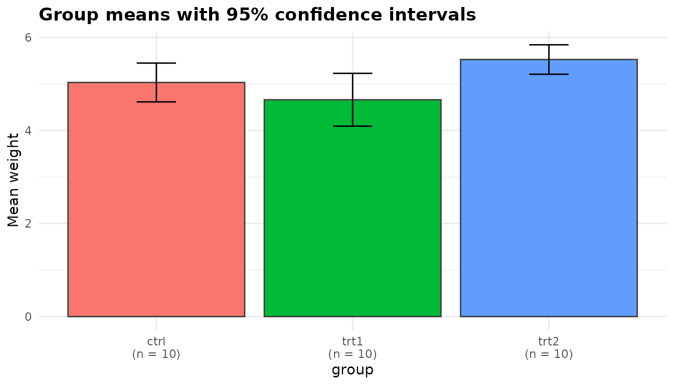

The means plot shows each group’s mean as a bar, with its 95% interval from $emmeans, and the group size under each label. Each interval is built from its own group’s standard deviation, so different widths reflect different spreads (and sizes). The intervals here are for the group means, not for the differences between them: two intervals that overlap do not mean the difference is non-significant. Read the comparisons from $posthoc.

plot(fit, "box")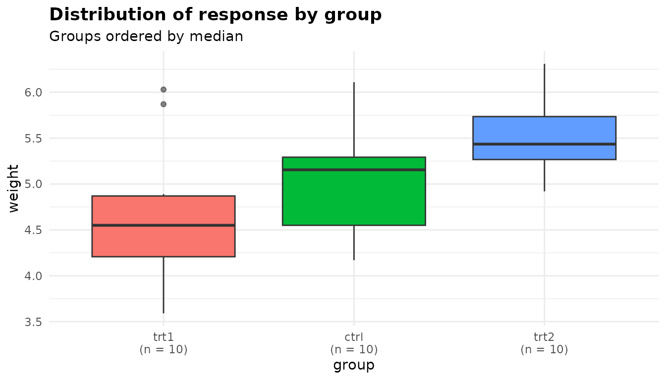

The box plot shows the raw distribution of each group, ordered by median and labelled with its size. This is where unequal spreads, skewness and outliers show up. Here trt1 is visibly more spread out than trt2, and two trt1 plants lie above its upper whisker.

plot(fit, "qq")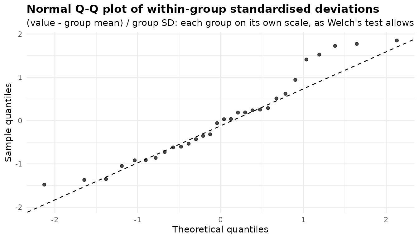

The qq plot is for normality. Each observation is expressed as its deviation from its own group’s mean, divided by its own group’s standard deviation, so every group contributes on its own scale, as Welch’s test allows. If the groups are roughly normal the points follow the dashed line. A bow away from the line suggests skewness, and a few isolated points far from it suggest outliers. Here the points follow the line closely through the middle. The largest few sit a little above it, among them the two high trt1 plants, at 1.52 and 1.72 standard deviations above their group mean. That is a hint of right skew, but departures of this size are common in 30 points drawn from a normal distribution.

Each plot is an ordinary ggplot object, so you can change it with +:

plot(fit, "box") +
  ggplot2::labs(title = "Dried weight by treatment", y = "Dried weight")

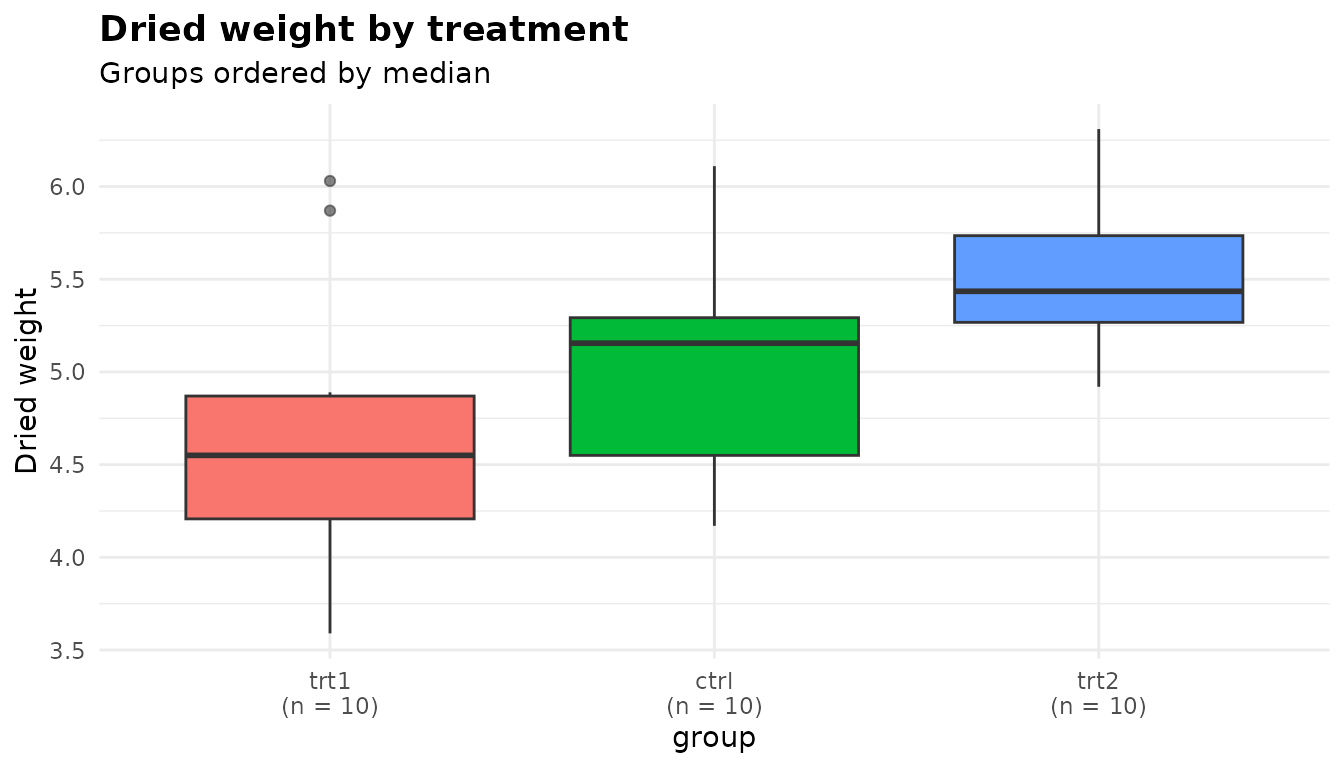
The plots article covers customisation in more detail.

Options worth knowing

`adjust`

adjust accepts any stats::p.adjust() method, spelled out in full: "holm" (the default), "hochberg", "hommel", "bonferroni", "BH", "BY", "fdr" or "none". Only p_adjusted changes. Holm controls the family-wise error rate and is never less powerful than Bonferroni. Benjamini-Hochberg ("BH") controls the false discovery rate instead, which suits screening many comparisons.

adj <- sapply(c("holm", "BH", "bonferroni", "none"), function(a)
  anova_welch(PlantGrowth, "weight", "group", adjust = a,
              plots = FALSE)$posthoc$p_adjusted)
cbind(fit$posthoc[, c("group1", "group2")], round(adj, 4))
#>   group1 group2   holm     BH bonferroni   none
#> 1   ctrl   trt1 0.2504 0.2504     0.7511 0.2504
#> 2   ctrl   trt2 0.0958 0.0718     0.1437 0.0479
#> 3   trt1   trt2 0.0279 0.0279     0.0279 0.0093

`conf_level`

conf_level sets the level of every interval the function returns: the group means, the pairwise differences and the standardised effect sizes (and the title of the means plot).

f90 <- anova_welch(PlantGrowth, "weight", "group", conf_level = 0.90)
f90$emmeans[, c("group", "mean", "conf_low", "conf_high")]
#>   group  mean conf_low conf_high
#> 1  ctrl 5.032 4.693993  5.370007
#> 2  trt1 4.661 4.200921  5.121079
#> 3  trt2 5.526 5.269449  5.782551
print(f90$effect_sizes[, c("group1", "group2", "hedges_g", "conf_low",
                           "conf_high")], digits = 3)
#>   group1 group2 hedges_g conf_low conf_high
#> 1   ctrl   trt1    0.508   -0.226     1.276
#> 2   ctrl   trt2   -0.911   -1.724    -0.158
#> 3   trt1   trt2   -1.273   -2.170    -0.482

Because the comparison intervals are per-comparison, one way to get Bonferroni-simultaneous intervals for all three differences is to ask for conf_level = 1 - 0.05 / 3. That widens the group-mean and effect-size intervals too.

`hedges_correction`

With hedges_correction = FALSE the effect size is the uncorrected standardised difference, and the column is named cohens_d. The intervals are unchanged, because they are for the population value either way.

d <- anova_welch(PlantGrowth, "weight", "group", hedges_correction = FALSE,
                 plots = FALSE)
print(d$effect_sizes[, c("group1", "group2", "cohens_d", "conf_low",
                         "conf_high")], digits = 3)
#>   group1 group2 cohens_d conf_low conf_high
#> 1   ctrl   trt1    0.533    -0.37   1.41993
#> 2   ctrl   trt2   -0.954    -1.88  -0.00867
#> 3   trt1   trt2   -1.346    -2.33  -0.32291

`posthoc`

There are choose(k, 2) pairs, so with many groups you may want only the omnibus test. The standardised differences are computed pair by pair alongside the comparisons, so posthoc = FALSE empties $effect_sizes too, and $notes says so:

np <- anova_welch(PlantGrowth, "weight", "group", posthoc = FALSE,
                  plots = FALSE)
np$notes
#> [1] "Pairwise comparisons were not computed (posthoc = FALSE); there would have been 3. $effect_sizes is empty for the same reason: Hedges' g is a per-pair quantity, computed with the comparisons."
is.null(np$effect_sizes)
#> [1] TRUE

Several grouping columns

warpbreaks counts the warp breaks per loom for two types of wool at three levels of tension. Given both columns, anova_welch() combines them into a single factor of the level combinations that contain data (unused combinations are dropped) and runs one Welch test across those cells:

wb <- anova_welch(warpbreaks, "breaks", c("wool", "tension"))
wb$anova
#>                   term statistic num_df   den_df     p_value
#> 1 wool x tension cells  4.555543      5 21.78918 0.005381049
wb$emmeans[, c("group", "n", "mean", "sd")]
#>   group n     mean        sd
#> 1 A : L 9 44.55556 18.097729
#> 2 B : L 9 28.22222  9.858724
#> 3 A : M 9 24.00000  8.660254
#> 4 B : M 9 28.77778  9.431036
#> 5 A : H 9 24.55556 10.272671
#> 6 B : H 9 18.77778  4.893306
wb$notes
#> [1] "The 2 grouping variables were combined into 6 cells and tested with a single omnibus Welch test. This cannot separate main effects or test an interaction; for that, use anova_glm() with interaction = TRUE."
#> [2] "Largest group variance is 13.7 times the smallest. Welch's test handles this; the classical F test would not."

The term reads wool x tension cells, and the cells are labelled A : L, B : L and so on. The test asks whether the six cell means are all equal. It cannot tell a wool effect from a tension effect, or test whether the effect of tension depends on the wool, and the first note says so. For that factorial question use anova_glm() with interaction = TRUE (walkthrough). The second note shows that the cell variances differ by a factor of more than 13, which is the situation Welch’s test is built for.

Two groups

With two groups the single pairwise comparison is the omnibus test: Welch’s F is the square of the Welch t, the p-values are identical, and no adjustment is applied.

f2g <- anova_welch(two, "weight", "group", plots = FALSE)
f2g$anova
#>    term statistic num_df   den_df   p_value
#> 1 group  1.419101      1 16.52359 0.2503825
f2g$posthoc[, c("statistic", "df", "p_value", "p_adjusted")]
#>   statistic       df   p_value p_adjusted
#> 1   1.19126 16.52359 0.2503825  0.2503825
f2g$notes
#> [1] "With two groups the pairwise comparison is the omnibus test; no multiplicity adjustment was needed."

What the notes say

fit$notes
#> character(0)

For the PlantGrowth fit, $notes is empty. No rows were dropped, every group was large enough for its Shapiro-Wilk test, the variance ratio was below 4, there was one grouping column, and there were more than two groups. Each of those would otherwise have produced a note. You have seen several above: the variance ratio (InsectSprays), combined cells (warpbreaks), two groups, and posthoc = FALSE. The function also writes a note if you ask for a low conf_level with very small groups and the bias-corrected estimate falls outside its own interval. Read $notes on every fit, including when you expect it to be empty.

Reporting the result

A write-up built from the fit with inline R, so that the numbers cannot drift from the analysis:

Dried plant weight differed between the three conditions (Welch’s F(2, 17.13) = 5.18, p = 0.017). In pairwise Welch t tests with Holm’s adjustment, plants given treatment 2 were heavier than those given treatment 1 by 0.865 (95% CI 0.249 to 1.481; Hedges’ g on the average-variance standard deviation = 1.27, 95% CI 0.32 to 2.33; adjusted p = 0.028). Neither treatment differed clearly from the control after adjustment (treatment 1: adjusted p = 0.250; treatment 2: adjusted p = 0.096).

The signs are flipped from the table so that the sentence reads “treatment 2 minus treatment 1”. State which standardiser you used: a Hedges’ g on the pooled standard deviation is a different quantity.